A constant- model assumes that the attenuation coefficient is linear in frequency (Kjartansson, 1979).
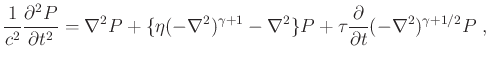
The time-domain viscoacoustic wave equation for constant- model can be written as (Carcione et al., 2002)
model assumes that the attenuation coefficient is linear in frequency (Kjartansson, 1979).
The time-domain viscoacoustic wave equation for constant- model can be written as (Carcione et al., 2002)
 |
(1) |
where
 is the spatial coordinate vector,
 is the pressure wavefield,
 |
(2) |
is a dimensionless parameter,  is the Laplacian operator,
 |
(3) |
and
 is the velocity model defined at the reference frequency
  . When is finite,
  is greater than zero, and the wave equation involves a fractional time derivative.
In a homogeneous medium, considering the plane-wave solution
 , where
  is the angular frequency and
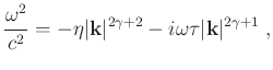
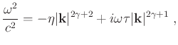
 is the complex wavenumber vector and substituting it into equation 1, leads to the dispersion relation
 |
(4) |
Starting from equation 4, Zhu and Harris (2014) derived the following approximate dispersion relation:
 |
(5) |
which corresponds to the following constant- wave equation with fractional Laplacians:
 |
|
|
(6) |
where
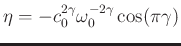 and
and
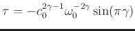 . Note that both
  (the phase velocity) and (the fractional power) can be heterogeneous (depending on
). Solving for in equation 5 yields:
(the phase velocity) and (the fractional power) can be heterogeneous (depending on
). Solving for in equation 5 yields:
 |
(7) |
where:
The phase function
 that determines the phase shift of wavefield for propagation in time is then defined as
 |
(10) |
and can be supplied to the low-rank one-step wave extrapolation algorithm (Sun and Fomel, 2013).
To compensate for attenuation, reversing the sign of the second term on the right hand side of equation 5 can amplify the amplitude, while the other term must be kept unchanged to counteract the dispersion effects (Zhu, 2014). Thus, the attenuation-compensated constant- wave equation corresponds to the dispersion relation:
 |
(11) |
which defines the complex-conjugate phase function:
 |
(12) |
Both  and
and  involve the fractional power of wavenumber, and depend on both
and
involve the fractional power of wavenumber, and depend on both
and
 , the Fourier transform pair. The low-rank one-step wave extrapolation operator (Sun and Fomel, 2013) provides a convenient way to utilize the phase function to extrapolate a viscoacoustic wavefield, while allowing
 , the fractional power coefficient, to vary in space. The one-step mixed-domain operator has the form of the following Fourier integral operator:
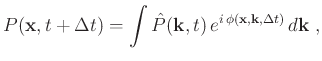 |
(13) |
where  is the spatial Fourier transform of
  .
Its adjoint form can be expressed as
.
Its adjoint form can be expressed as
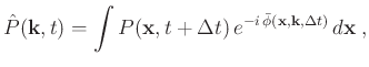 |
(14) |
where
 denotes the complex conjugate of
  . Substituting equation 10 into equation 13, we can write the forward extrapolation operator explicitly as
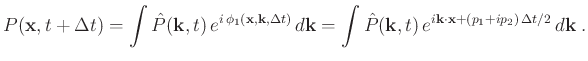 |
|
|
(15) |
The corresponding adjoint operator takes the form:
 |
|
|
(16) |
To make the computation feasible, we apply low-rank decomposition proposed by Fomel et al. (2013) to approximate the wave extrapolation symbol in equations 15 and 16.
Note that the adjoint operator compensates for velocity dispersion. Because the sign of  remains unchanged, the amplitude of waves will be attenuated during backward propagation using equation 16. This means that the adjoint operator may not be well suited for RTM because the backward wavefield would be attenuated twice. However, the adjoint operator can be supplied into the framework of least-squares RTM which can then iteratively recover the amplitude loss caused by viscoacoustic attenuation (Sun et al., 2014).
An alternative strategy for backward wave propagation is to try compensating for the full attenuation effect (both amplitude loss and velocity dispersion) using the operator
 |
(17) |
which is the adjoint of
 |
(18) |
In application to RTM, operator in equation 17 has an exponentially growing term which can amplify the energy in the forward-propagated source wavefield. In the same manner, operator in equation 18 can compensate for the amplitude loss in the backward-propagated receiver wavefield. In order to avoid magnifying high-frequency components during wave propagation, we employ a low-pass Tukey filter for the attenuation and dispersion operators in the wavenumber domain (Zhu et al., 2014). A complex-valued imaging condition that compensates for both velocity dispersion and amplitude loss can be obtained by cross-correlating the source and receiver wavefields modeled by equations 17 and 18 (Zhu et al., 2014).
In this way, the migrated viscoacoustic data gets corrected for attenuation due to viscoacoustic material encountered along the wave path. As will be demonstrated in the numerical examples, -compensated RTM is capable of enhancing illumination in areas where attenuating material is present. For a more accurate compensation of attenuation, operators 17 and 18 can be used to design a preconditioner in iterative least-squares RTM.
2019-07-17