Full-waveform inversion using seislet regularization

Theory

The objective function of standard FWI can be written as

$$J(\mathbf{m})=\frac{1}{2} \vert\vert\mathbf{d}_ -\mathbf{F}(\mathbf{m})\vert\vert _2^2 \; ,$$ (1)

where $\mathbf{m}$ is the velocity model, $\mathbf{d}_$obs is the observed waveform data and $\mathbf{F}$ stands for the nonlinear forward modeling operator.

A popular local optimization algorithm for minimizing this function is based on the nonlinear conjugate-gradient method (Tarantola, 1987; Mora, 1987), where the model is updated at the iteration $n$ in the direction of $\mathbf{s}_n$ , which is a linear combination of the gradient at iteration $n$ , $\nabla J(\mathbf{m}_n)$ , and the previous conjugate direction $\mathbf{s}_{n-1}$ . This optimization scheme can be formulated as follows:

$$\mathbf{m}_{n+1}=\mathbf{m}_n + \alpha_n \mathbf{s}_n \; , \quad \mathbf{s}_n=-\nabla J(\mathbf{m}_n)+ \beta_n \mathbf{s}_{n-1} \;,$$ (2)

where scalar $\alpha_n$ can be obtained by perfoming a line search and $\beta_n$ is designed to guarantee that $\mathbf{s}_n$ and $\mathbf{s}_{n-1}$ are conjugate.

We propose to apply nonlinear shaping regularization (Fomel, 2008) to impose sparseness of the velocity model in the seislet domain and modify the iteration process in equation 2 as follows:

$$\mathbf{m}_{n+1}=\mathbf{S}^{-1}\mathbf{T}\mathbf{S}(\mathbf{m}_n + \alpha_n \mathbf{s}_n) \; ,$$ (3)

where $\mathbf{S}^{-1}$ and $\mathbf{S}$ stand for the inverse and forward seislet transforms, respectively. $\mathbf{T}$ is the soft thresholding operator and has the following function expression:

$$T(x)= \begin{cases}x-t \;, & x>t \\ 0 \;, & \vert x\vert \le t \\ x+t \;, & x<-t \end{cases}$$ (4)

where $t$ is a positive threshold level. If seislet transform were an unitary operator, the iteration process in equation 3 would be equivalent to using linearized Bregman iteration (Cai et al., 2009; Yin et al., 2008) to minimize the following objective function:

$$J(\mathbf{m})=\frac{1}{2} \vert\vert\mathbf{d}_ -\mathbf{F}(\mathbf{m})\vert\vert _2^2 + \lambda \vert\vert\mathbf{S}\mathbf{m}\vert\vert _1 \; ,$$ (5)

where $\lambda$ is a regularization parameter.

The difference of equation 3 to the iterative scheme described by equation 2 is that the new scheme involves a model shaping operator, which is the combination of inverse seislet transform, soft thresholding operator and forward seislet transform. The purpose of the shaping operator $\mathbf{S}^{-1}\mathbf{T}\mathbf{S}$ is to remove possible artifacts existing in the updated model and to gradually achieve a geologically meaningful model. In implementation of equation 3, step length $\alpha_n$ is estimated by line search without including the shaping operator, and we apply the shaping operator to the updated model after line search to get the new model $\mathbf{m}_{n+1}$ . In this way, we just use the shaping operator once at each iteration.

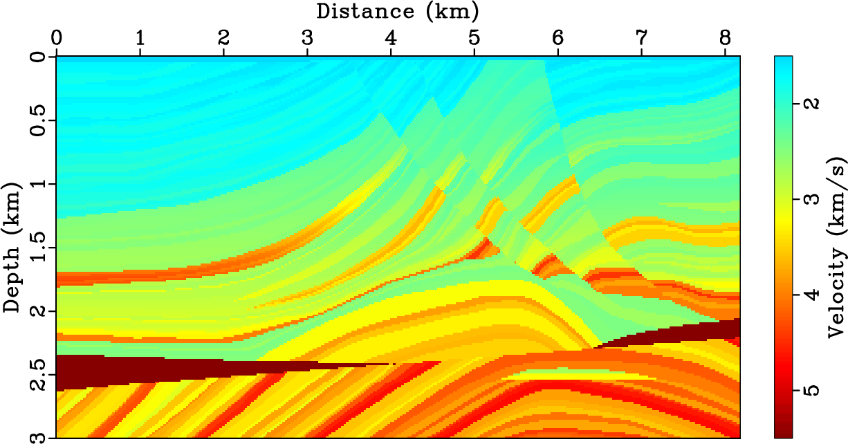
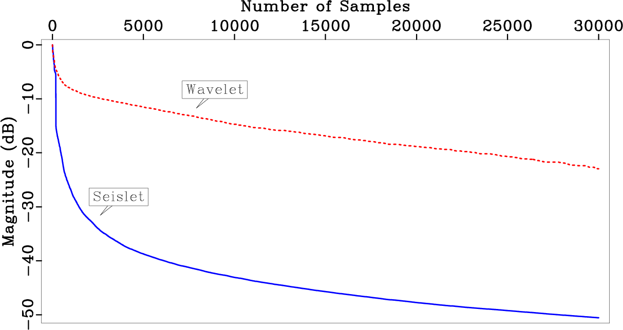
Seislet transform requires the input of local slope, because in the seislet domain, the model is represented by the basis functions that are aligned with local structures. Figure 1 shows a simple test to check the properties of velocity model in the seislet domain. We compare seislet coefficients and basis functions with those of the digital wavelet transform, using the Marmousi model (Figure 1a). The dip required by seislet transform is directly estimated from the Marmousi model in this test. Figure 1b and 1c show the Marmousi model in the wavelet and seislet domain, respectively. We observe that the non-zero seislet coefficients focus at coarse scales but wavelet transform has small residual coefficients at fine scales. From this observation, we can conclude that the seislet transform has a better data compression and sparsity than the wavelet transform, which is further verified by Figure 1d, where a significantly faster decay of the seislet coefficients is evident. Figure 1e and 1f show some randomly selected representative basis functions for wavelet and seislet transforms, respectively. We can observe that the direction of seislet basis functions follows structural direction, while the wavelet basis functions correspond to zero slope.

marm,wavelet,seislet,comparison,impw,imps
Figure 1. Coefficients and basis functions of wavelet and seislet transforms for the Marmousi model. (a) The exact Marmousi model; (b) model in the wavelet domain; (c) model in the seislet domain; (d) transform coefficients sorted from large to small, normalized, and plotted on a decibel scale; (e) and (f) randomly selected representative basis functions for wavelet and seislet transforms, respectively.

Full-waveform inversion using seislet regularization