|
|
|
|
Next: Viscoacoustic RTM and RTDM Up: Theory Previous: Theory
|
|
|
|
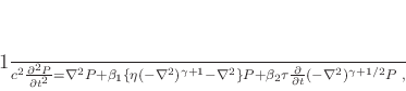
A constant-![]() model (Kjartansson, 1979) describes an attenuating medium whose quality factor
model (Kjartansson, 1979) describes an attenuating medium whose quality factor ![]() is constant in frequency (but may vary in space), indicating that the attenuation coefficient is linear in frequency. Zhu and Harris (2014) derived the following approximate constant-
is constant in frequency (but may vary in space), indicating that the attenuation coefficient is linear in frequency. Zhu and Harris (2014) derived the following approximate constant-![]() wave equation with decoupled fractional Laplacians for modeling and imaging in viscoacoustic media:
wave equation with decoupled fractional Laplacians for modeling and imaging in viscoacoustic media:
| (2) | |||
| (3) | |||
| (4) | |||
| (5) |
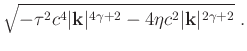
Setting both ![]() and
and ![]() to one, equation 1 leads to the viscoacoustic dispersion relation with fractional powers of the wave number:
to one, equation 1 leads to the viscoacoustic dispersion relation with fractional powers of the wave number:
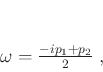
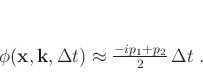
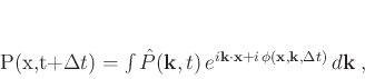
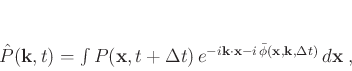
The one-step wave extrapolation provides an approximate solution to equation 1 by incorporating the phase function defined in equation 10 into the Fourier integral operator (FIO):
The FIOs introduced in equations 11 and 12 can be efficiently applied using the lowrank one-step wave extrapolation Sun et al. (2015), which we also refer to as the lowrank PSPI operator because of its resemblance to the well-known PSPI method for solving the one-way wave equation (Gazdag and Squazzero, 1984; Margrave and Ferguson, 1999; Kesinger, 1992). The detailed formulation of lowrank PSPI operator, as well as the derivation of its adjoint operator, the lowrank NSPS operator, is shown in the appendix. RTM and LSRTM in viscoacoustic media can therefore be constructed using the forward and adjoint operators.
|
|
|
|