|
|
|
|
On anelliptic approximations for |
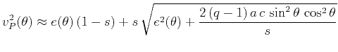
Despite the beautiful symmetry of Muir's approximations (12) and (17), they are less accurate in practice than some other approximations, most notably the weak anisotropy approximation of Thomsen (1986), which can be written as (Tsvankin, 1996)
Note that both approximations involve the anellipticity factor (![]() or
or
![]() ) in a linear fashion. If the anellipticity effect is
significant, the accuracy of Muir's equations can be improved by
replacing the linear approximation with a nonlinear one. There are, of
course, infinitely many nonlinear expressions that share the same
linearization. In this study, I focus on the shifted hyperbola approximation,
which follows from the fact that an expression of the form
) in a linear fashion. If the anellipticity effect is
significant, the accuracy of Muir's equations can be improved by
replacing the linear approximation with a nonlinear one. There are, of
course, infinitely many nonlinear expressions that share the same
linearization. In this study, I focus on the shifted hyperbola approximation,
which follows from the fact that an expression of the form
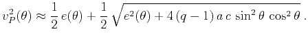
Thus, we seek an approximation of the form
One can verify that the velocity curvature
![]() around the
vertical axis
around the
vertical axis ![]() for approximation (24) depends on the
chosen value of
for approximation (24) depends on the
chosen value of ![]() but does not depend on the value of the shift parameter
but does not depend on the value of the shift parameter
![]() . This means that the velocity profile
. This means that the velocity profile
![]() becomes sensitive to
becomes sensitive to
![]() only further away from the vertical direction. This separation of
influence between the approximation parameters is an important and attractive
property of the shifted hyperbola approximation. I find an appropriate value
for
only further away from the vertical direction. This separation of
influence between the approximation parameters is an important and attractive
property of the shifted hyperbola approximation. I find an appropriate value
for ![]() by fitting additionally the fourth-order derivative
by fitting additionally the fourth-order derivative
![]() at
at ![]() to the corresponding derivative of the exact
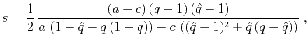
expression. The fit is achieved when
to the corresponding derivative of the exact
expression. The fit is achieved when ![]() has the value
has the value
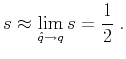
Approximation (28) is exactly equivalent to the acoustic
approximation of Alkhalifah (1998,2000a),
derived with a different set of parameters by formally setting the ![]() -wave
velocity (
-wave
velocity (![]() ) in equation (4) to zero. A similar
approximation is analyzed by Stopin (2001).
Approximation (28) was proved to possess a remarkable accuracy
even for large phase angles and significant amounts of anisotropy.
Figure 3 compares the accuracy of different approximations using
the parameters of the Greenhorn shale. The acoustic approximation appears
especially accurate for phase angles up to about 25 degrees and does not
exceed the relative error of 0.3% even for larger angles.
) in equation (4) to zero. A similar
approximation is analyzed by Stopin (2001).
Approximation (28) was proved to possess a remarkable accuracy
even for large phase angles and significant amounts of anisotropy.
Figure 3 compares the accuracy of different approximations using
the parameters of the Greenhorn shale. The acoustic approximation appears
especially accurate for phase angles up to about 25 degrees and does not
exceed the relative error of 0.3% even for larger angles.

|
|---|
|
errphp
Figure 3. Relative error of different phase velocity approximations for the Greenhorn shale anisotropy. Short dash: Thomsen's weak anisotropy approximation. Long dash: Muir's approximation. Solid line: suggested approximation (similar to Alkhalifah's acoustic approximation.) |
|
|
|
|
|
|
On anelliptic approximations for |
 and
and