On anelliptic approximations for $qP$ velocities in transversally isotropic media

Application: Finite-difference traveltime computation

As an essential part of seismic imaging with the Kirchhoff method, traveltime computation has received a lot of attention in the geophysical literature. Finite-difference eikonal solvers (Podvin and Lecomte, 1991; Vidale, 1990; van Trier and Symes, 1991) provide an efficient and convenient way of computing first arrival traveltimes on regular grids. Although they have a limited capacity for imaging complex structures (Geoltrain and Brac, 1993), eikonal solvers can be extended in several different ways to accommodate multiple arrivals (Bevc, 1997; Abgrall and Benamou, 1999; Symes, 1998). A particularly attractive approach to finite-difference traveltime computation is the fast marching method, developed by Sethian (1996) in the general context of level set methods for propagating interfaces (Sethian, 1999; Osher and Sethian, 1988). Sethian and Popovici (1999) adopt the fast marching method for computing seismic isotropic traveltimes. Alternative implementations are discussed by Sun and Fomel (1998), Alkhalifah and Fomel (2001), and Kim (2002). The fast marching method possesses a remarkable numerical stability, which results from a cleverly chosen order of finite-difference evaluation. The order selection scheme resembles expanding wavefronts of Qin et al. (1992) and wavefront tracking of Cao and Greenhalgh (1994).

While the anisotropic eikonal equation (1) operates with phase velocities, the kernel of the fast marching eikonal solver can be interpreted in terms of local ray tracing in a constant-velocity background (Fomel, 1997) and is more conveniently formulated with the help of the group velocity. Sethian and Vladi-mirsky (2001) present a thorough extention of the fast marching method to anisotropic wavefront propagation in the form of ordered upwind methods. In this paper, I adopt a simplified approach. Anisotropic traveltimes are computed in relation to an isotropic background. At each step of the isotropic fast marching method, the local propagation direction is identified, and the anisotropic traveltimes are computed by local ray tracing with the group velocity corresponding to the same direction. This is analogous to the tomographic linearization approach in ray tracing, where anisotropic traveltimes are computed along ray trajectories, traced in the isotropic background (Chapman and Pratt, 1992). Alkhalifah (2002) and Schneider (2003) present different approaches for linearizing the anisotropic eikonal equation.

Many alternative forms of finite-difference traveltime computation in anisotropic media are presented in the literature (Perez and Bancroft, 2001; Dellinger and Symes, 1997; Qin and Schuster, 1993; Zhang et al., 2002; Qin and Symes, 2002; Kim, 1999; Bousquie and Siliqi, 2001). Although the method of this paper has limited accuracy because of the linearization assumption, it is simple and efficient in practice and serves as an illustration for the advantages of the explicit group velocity approximation (33). For a more accurate and robust extension of the fast marching method for anisotropic traveltime calculation, I recommend the ordered upwind methods of Sethian and Vladi-mirsky (2001,2003).

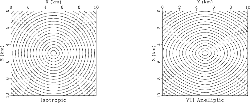
Figure 8 shows finite-difference wavefronts for an isotropic and an anisotropic homogeneous media, compared with the exact solutions. The anisotropic media has the parameters of the Greenhorn shale. The finite-difference error decreases with finer sampling.

const
Figure 8. Finite-difference wavefronts in an isotropic (left) and an anisotropic (right) homogeneous media. The anisotropic media has the parameters of the Greenhorn shale. The finite-difference sampling is 100 m. The contour sampling is 0.1 s. Dashed curves indicate the exact solution. The finite-difference error will be reduced at finer sampling.

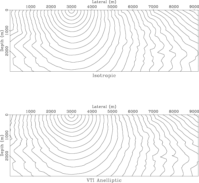
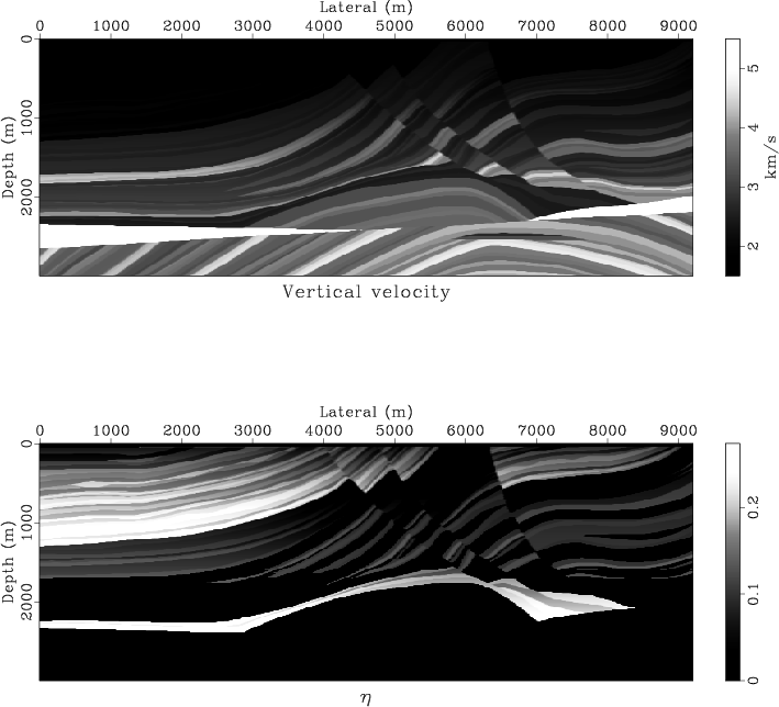
Figure 9 shows the first arrival wavefronts (traveltime contours) computed in the anisotropic Marmousi model created by Alkhalifah (1997) in comparison with wavefronts for the isotropic Marmousi model (TME, 1990; Versteeg, 1994). The model parameters are shown in Figure 10. The observed significant difference in the wavefront position suggests a difference in the positioning of seismic images when anisotropy is not properly taken into account.

marm
Figure 9. Finite-difference wavefronts in the isotropic (top) and anisotropic (bottom) Marmousi models. A significant shift in the wavefront position suggest possible positioning error when seismic imaging does not take anisotropy into account.

marmmod
Figure 10. Alkhalifah's anisotropic Marmousi model. Top: vertical velocity. Bottom: anelliptic $\eta$ parameter. The vertical velocity is taken equal to the NMO velocity $V_n$ .

On anelliptic approximations for $qP$ velocities in transversally isotropic media