|
 |
 |
 | Generalized nonhyperbolic moveout approximation |  |
![[pdf]](icons/pdf.png) |
Next: Bibliography
Up: Fomel & Stovas: Generalized
Previous: Appendix D: REFLECTION FROM
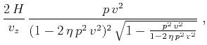
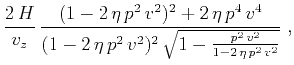
According to the acoustic approximation of
Alkhalifah (1998), one can use the following parametric
equations to define the traveltime-offset relationship in a
homogeneous VTI model:
where  is the ray parameter,
  is the depth of the reflector,
 is the vertical velocity,
  is the NMO velocity, and
  is
the dimensionless parameter introduced by Alkhalifah and Tsvankin (1995).
is
the dimensionless parameter introduced by Alkhalifah and Tsvankin (1995).
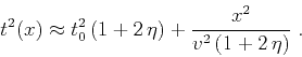
At small offsets, the homogeneous VTI traveltime behaves as
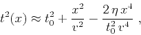 |
(80) |
which allows us to define  according to equation 18.
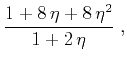
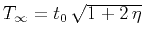
At large offsets, the homogeneous VTI traveltime behaves as
 |
(81) |
Comparing with equation 24, we note that
 and
and
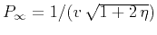 . Substituting into
equations 25-26, we derive the coefficients
. Substituting into
equations 25-26, we derive the coefficients  and
and
 to be
to be
|
|
|
|
| Generalized nonhyperbolic moveout approximation | |
|
Next: Bibliography
Up: Fomel & Stovas: Generalized
Previous: Appendix D: REFLECTION FROM
2013-07-26