Seismic data decomposition into spectral components using regularized nonstationary autoregression

Benchmark tests

sig,tf,group
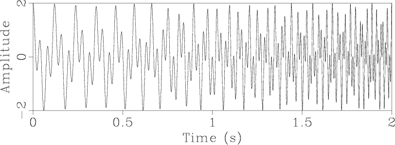
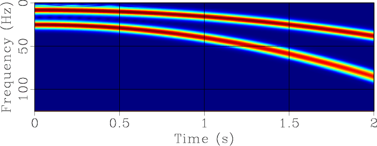
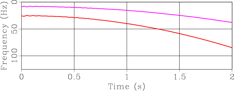
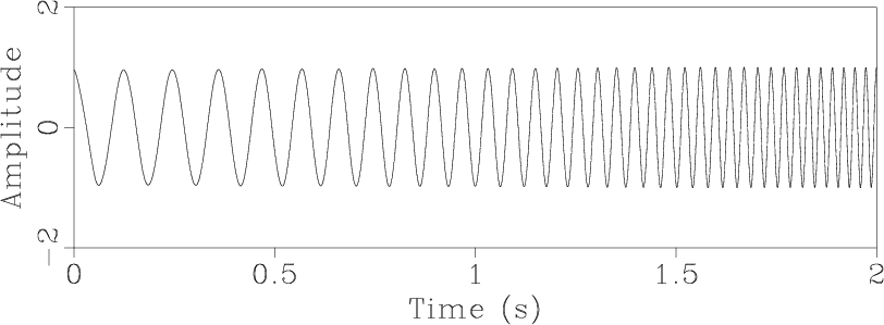
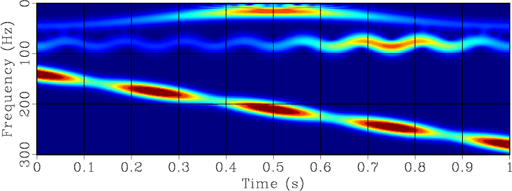
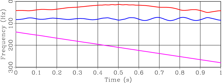
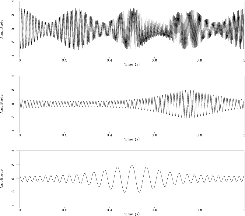
Figure 1. (a) Test signal from Liu et al. (2011) composed of two variable-frequency components. (b) Time-frequency decomposition. (c) Instantaneous frequencies estimated by RNAR.

sign1,sign2
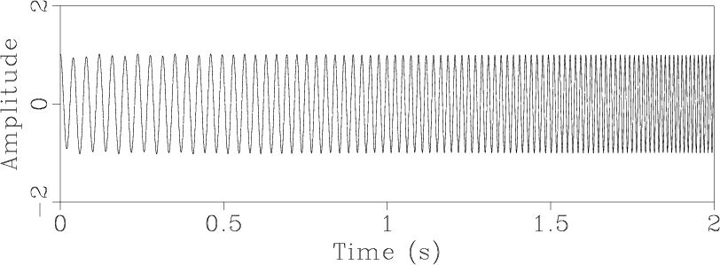
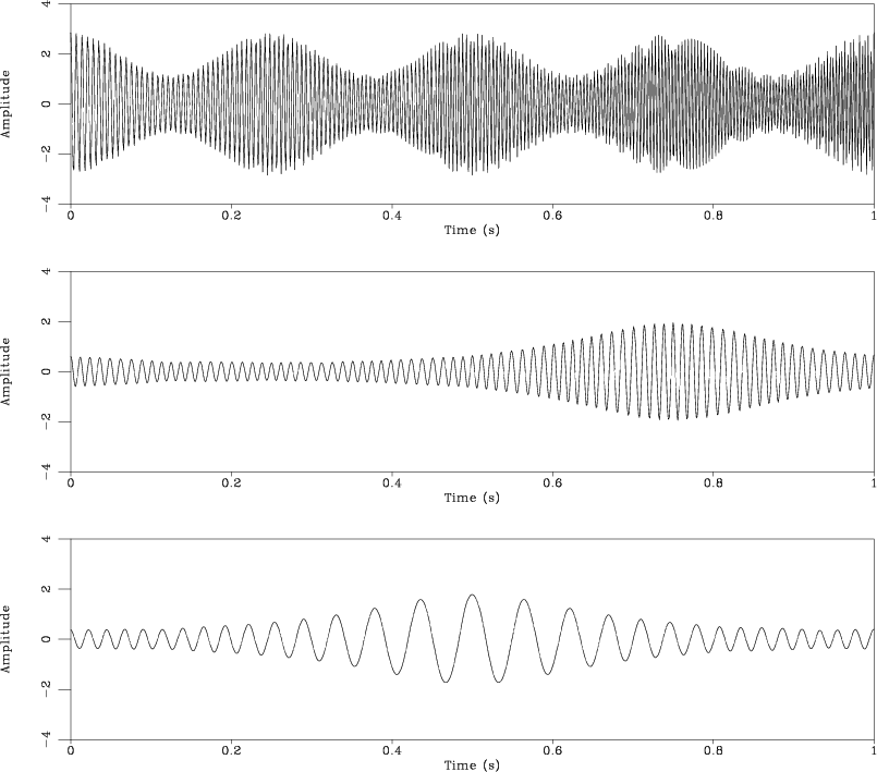
Figure 2. Decomposition of the signal from Figure 1a into two spectral components using RNR.

Figure 1a shows a benchmark signal from Liu et al. (2011), which consists of two nonstationary components with smoothly varying (parabolic) frequencies. The corresponding time-frequency analysis over a range of regularly sampled frequencies is shown in Figure 1b. Two instantaneous frequencies were extracted at Step 2 of the algorithm from a time-varying, three-point prediction-error filter (Figure 1c). They correspond precisely to the two components present in the synthetic signal. Finally, Step 3 separates these components (Figure 2.)

msig,mtf,mgroup
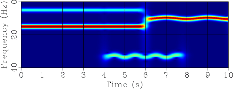
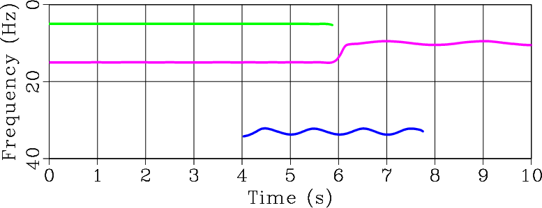
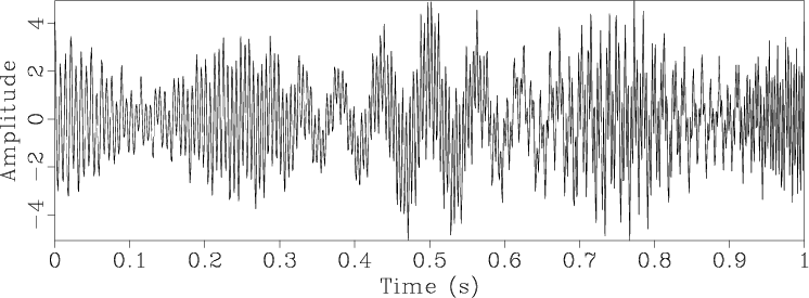
Figure 3. (a) Test signal from Herrera et al. (2013) composed of several variable-frequency components. (b) Time-frequency decomposition. (c) Instantaneous frequencies estimated by RNAR.

narall
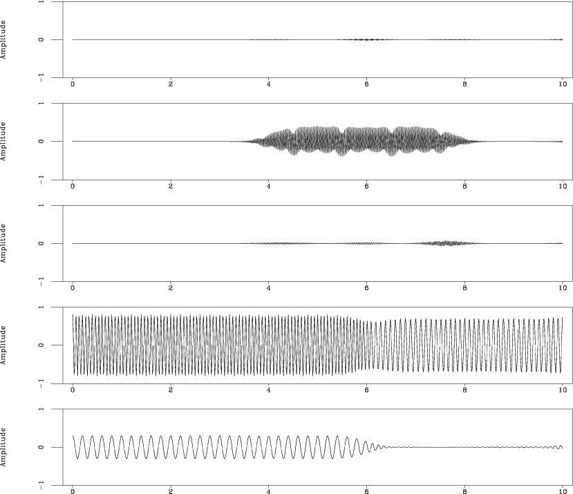
Figure 4. Decomposition of the signal from Figure 3a into spectral components using RNR. The components are sorted in the order of decreasing frequency.

emd
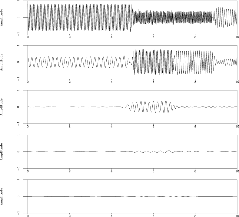
Figure 5. Decomposition of the signal from Figure 3a into intrinsic mode functions using EMD. Compare with Figure 4.

The next benchmark example is taken from Herrera et al. (2013). Figure 3a shows the input signal, which is composed of several components with variable frequencies. The components can be identified in the time-frequency decomposition analysis (Figure 3b) generated with the method of Liu et al. (2011). More directly, they are extracted using RNAR (the method of this paper), with the output shown in Figure 3c. Fitting a sum of different components to the data by RNR, we can estimate their respective amplitudes. The output is shown in Figure 4. For comparison, I show the output of EMD (empirical mode decomposition) in Figure 5. For robustness, I used EEMD (ensemble EMD) suggested by Wu and Huang (2009). Although EEMD succeeds in separating the signal into components with variable frequencies, the individual components are not as meaningful as those identified by RNAR.

hsig,htf,hgroup
Figure 6. (a) Test signal from Hou and Shi (2013) composed of several variable-frequency and variable-amplitude components. (b) Time-frequency decomposition. (c) Instantaneous frequencies estimated by RNAR.

sigs
Figure 7. Signal components making the signal in Figure 6a.

nar
Figure 8. Decomposition of the signal from Figure 6a into spectral components using RNR.

hfit
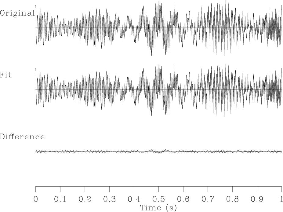
Figure 9. Fitting the signal from Figure 6a with the sum of three components shown in Figure 8.

The third benchmark test is taken from Hou and Shi (2013). The signal in this case (Figure 6a) consists of three components with variable frequencies and amplitudes (Figure 7). RNAR correctly identifies the three components (Figure 6c) that are also visible on the time-frequency plot (Figure 6b). Next, RNR extracts the three components (Figure 8) by fitting their sum to the data (Figure 9) and adjusting the amplitudes. The sparse inversion algorithm proposed by Hou and Shi (2013) achieves a more accurate result in this case but at a much higher computational cost.

Seismic data decomposition into spectral components using regularized nonstationary autoregression