Lowrank one-step wave extrapolation for reverse-time migration

Two-layer Model

twolayer,fwavefd,wave1-2,wave2-2,wave1-3,wave2-3,wave1-10,wave1-20,wave1-30
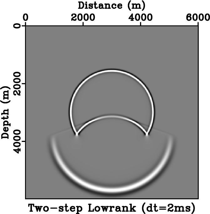
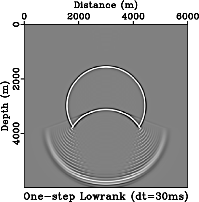
Figure 5. Stability comparison between different schemes. Wavefield snapshots are taken at $t=1.1\;s$ . (a) Two-layer velocity model. Velocity is $1500\;m/s$ in the top layer and $4500\;m/s$ in the bottom layer. (b) Wavefield modeled by FD with $\Delta t=2\;ms$ . (c) Wavefield modeled by the one-step scheme with $\Delta t=2\;ms$ . (d) Wavefield modeled by the two-step scheme with $\Delta t=2\;ms$ . (e) Wavefield modeled by the one-step scheme with $\Delta t=3\;ms$ . (f) Wavefield modeled by the two-step scheme with $\Delta t=3\;ms$ . (g) Wavefield modeled by the one-step scheme with $\Delta t=10\;ms$ . (h) Wavefield modeled by the one-step scheme with $\Delta t=20\;ms$ . (i) Wavefield modeled by the one-step scheme with $\Delta t=30\;ms$ .

We use a simple two-layer velocity model similar to the one used by Du et al. (2014) to demonstrate the stability of one-step wave extrapolation using lowrank approximation. Figure 5 shows the comparison among the stability of lowrank one-step, lowrank two-step and fourth-order FD methods. The velocity model has a sharp contrast at the depth of $3795\;m$ ; the upper layer has a velocity of $1500\;m/s$ , and the lower layer has a velocity of $4500\;m/s$ (Figure 5a). The model is discretized on a $400 \times 400$ grid with a spacing of $15\;m$ along both horizontal and vertical directions. An explosive source, with a Ricker wavelet using a peak frequency of $16\;Hz$ (maximum frequency approximately $50\;Hz$ ) is injected in the center of the model. When a time step of $2\;ms$ is used, the classic fourth-order FD method suffers from visible dispersion artifacts (Figure 5b), whereas both the one-step and two-step schemes produce waves free of artifacts (Figure 5c and 5d). When a time step of $3\;ms$ is used, the one-step scheme is stable (Figure 5e) whereas the two-step scheme starts to develop artifacts near the velocity contrast (Figure 5f). The FD method is no longer stable and therefore is not plotted. At $10\;ms$ , which corresponds to the Nyquist sampling rate, the one-step scheme remains stable (Figure 5g), but the two-step scheme becomes unstable and thus is not plotted. Using $20\;ms$ , the one-step scheme is still stable, but starts to develop ringing artifacts similar to those observed by Du et al. (2014) (Figure 5h). Using the time step size of $30\;ms$ , the ringing effects aggravate, however the operator remains stable (Figure 5i).

Lowrank one-step wave extrapolation for reverse-time migration