|
|
|
|
Lowrank one-step wave extrapolation for reverse-time migration |


|
|---|
|
vp,vx,eta,theta
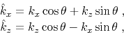
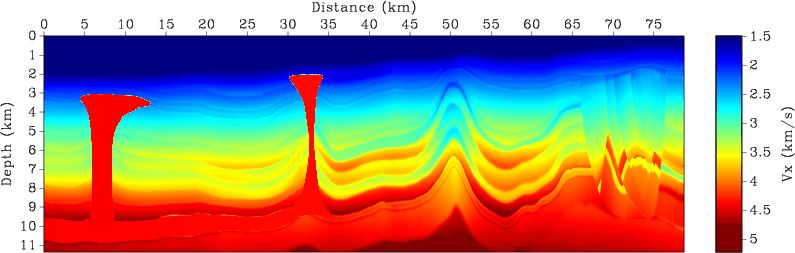
Figure 11. BP-2007 anisotropic benchmark model. (a) P-wave phase velocity along the axis of symmetry |
|
|


|
|---|
|
wavesnaps-4,wavesnaps-10,wavesnaps-20,wavesnaps-30
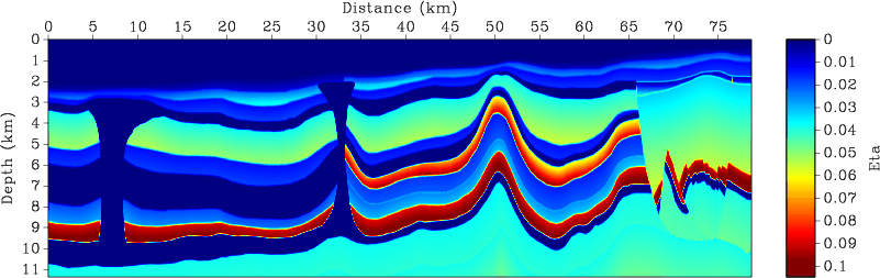
Figure 12. Wavefield snapshots taken at different times showing P-wave propagation through the 2007 BP TTI model. Propagation-direction-dependent absorbing boundary conditions allow little energy to be reflected, even at wide-incident angles. The four wavefield snapshots calculated using different time step sizes are almost identical: (a) |
|
|


|
|---|
|
swavesnaps-2,swavesnaps-4,swavesnaps-10,swavesnaps-20
Figure 13. Wavefield snapshots taken at different times showing S-wave propagation through the 2007 BP TTI model. The four wavefield snapshots calculated using different time step sizes are almost identical: (a) |
|
|
To show that the proposed method handles anisotropic media accurately, we propagate qP- and qSV-waves in a portion of the 2007 anisotropic benchmark model from BP. The model has a horizontal spacing of ![]() and a vertical spacing of
and a vertical spacing of ![]() . As shown in Figure 11, the model exhibits a strong tilted transverse isotropy (TTI). We restrict the modeled area between
. As shown in Figure 11, the model exhibits a strong tilted transverse isotropy (TTI). We restrict the modeled area between ![]() and
and ![]() . Since the original model does not include S-wave velocity, we compute a vertical S-wave velocity profile simply as
. Since the original model does not include S-wave velocity, we compute a vertical S-wave velocity profile simply as ![]() times the original vertical P-wave velocity.
times the original vertical P-wave velocity.
To calculate the qP- and qSV-wave phase velocities, we employ the exact formulas defined by Gassmann (1964):
To mimic an unbounded medium, we apply the absorbing boundary condition in equation 26. First, a time step size of ![]() for qP-wave and
for qP-wave and ![]() for qSV-wave is used. A Ricker wavelet source with a peak frequency of
for qSV-wave is used. A Ricker wavelet source with a peak frequency of ![]() is located at
is located at
![]() and
and
![]() . Figures 12a and 13a illustrates wavefield snapshots taken at different times overlaid on top of each other. Because of the accumulative effect of the large time step, model complexity and extra anisotropy introduced by the absorbing boundary conditions, the lowrank approximation took
. Figures 12a and 13a illustrates wavefield snapshots taken at different times overlaid on top of each other. Because of the accumulative effect of the large time step, model complexity and extra anisotropy introduced by the absorbing boundary conditions, the lowrank approximation took ![]() for qP-wave and
for qP-wave and ![]() for qSV-wave for an accuracy threshold of
for qSV-wave for an accuracy threshold of
![]() .
.
To test the effect of using large ![]() for wave propagation, we choose a series of increasing
for wave propagation, we choose a series of increasing ![]() while enforcing the same accuracy requirement (
while enforcing the same accuracy requirement (
![]() ). The qP-wave wavefields (Figure 12) generated using
). The qP-wave wavefields (Figure 12) generated using
![]() and
and ![]() are almost identical. Similarly, the qSV-wave wavefields (Figure 13) generated using
are almost identical. Similarly, the qSV-wave wavefields (Figure 13) generated using
![]() and
and ![]() have very little difference. This shows that the stability and accuracy of wave extrapolation is not compromised by using very large time steps, even beyond the Nyquist limit of
have very little difference. This shows that the stability and accuracy of wave extrapolation is not compromised by using very large time steps, even beyond the Nyquist limit of ![]() .
.
To investigate the effects of time step size (![]() ) and accuracy level (
) and accuracy level (![]() ) of lowrank approximation on the computational cost, which is directly controlled by the rank of the approximation, we conduct a series of experiments using different values of
) of lowrank approximation on the computational cost, which is directly controlled by the rank of the approximation, we conduct a series of experiments using different values of ![]() and
and ![]() for qP-wave propagation. No absorbing boundary condition is applied in this test. Table 1 lists rank
for qP-wave propagation. No absorbing boundary condition is applied in this test. Table 1 lists rank ![]() required by different time step sizes to achieve different accuracy levels. We can observe that the lowrank algorithm requires a higher rank to maintain the same level of accuracy when the time step size increases. On the other hand, with the same time step size, a higher rank may be needed to achieve a higher accuracy. In practice, we find that
required by different time step sizes to achieve different accuracy levels. We can observe that the lowrank algorithm requires a higher rank to maintain the same level of accuracy when the time step size increases. On the other hand, with the same time step size, a higher rank may be needed to achieve a higher accuracy. In practice, we find that
![]() is small enough to guarantee accurate wave kinematics. Since making a larger step in time requires a smaller number of steps, the optimal time step size
is small enough to guarantee accurate wave kinematics. Since making a larger step in time requires a smaller number of steps, the optimal time step size ![]() can be selected to be the one that minimizes the total number of Fast Fourier Transforms (FFTs) required to accomplish the modeling or imaging task at hand.
In practice, we found that this minimization problem usually has a straightforward solution: the larger
can be selected to be the one that minimizes the total number of Fast Fourier Transforms (FFTs) required to accomplish the modeling or imaging task at hand.
In practice, we found that this minimization problem usually has a straightforward solution: the larger ![]() is, the less computation is required. Therefore, the optimal solution will be the largest
is, the less computation is required. Therefore, the optimal solution will be the largest ![]() that satisfies other constraints, such as the imaging condition when performing RTM.
that satisfies other constraints, such as the imaging condition when performing RTM.
| 0.5 | 1 | 2 | 4 | 8 | 16 | 32 | 64 | |
| 4 | 7 | 7 | 10 | 14 | 19 | 33 | 53 | |
| 7 | 9 | 13 | 15 | 22 | 30 | 46 | 76 | |
| 11 | 14 | 18 | 23 | 30 | 43 | 59 | 84 |
|
|
|
|
Lowrank one-step wave extrapolation for reverse-time migration |
![$\displaystyle \frac{1}{2} \left[(c_{11}+c_{55}) \hat{k}_x + (c_{33}+c_{55}) \hat{k}_z\right] +$](img144.png)
![$\displaystyle \frac{1}{2} \sqrt{\left[(c_{11}-c_{55}) \hat{k}_x - (c_{33}-c_{55}) \hat{k}_z\right]^2 +
4 (c_{13}+c_{55})^2 \hat{k}_x \hat{k}_z}\;;$](img145.png)
![$\displaystyle \frac{1}{2} \left[(c_{11}+c_{55}) \hat{k}_x + (c_{33}+c_{55}) \hat{k}_z\right] -$](img147.png)
![$\displaystyle \frac{1}{2} \sqrt{\left[(c_{11}-c_{55}) \hat{k}_x -
(c_{33}-c_{55}) \hat{k}_z\right]^2 +
4 (c_{13}+c_{55})^2 \hat{k}_x \hat{k}_z}\;,$](img148.png)