Random noise attenuation using local signal-and-noise orthogonalization

Synthetic examples

We use two synthetic examples to test the performance of the proposed denoising algorithm. For consistency, we use denoising to denote random noise attenuation for regular seismic data, and deblending to denote blending noise attenuation for simultaneous-source seismic data. The first example is a deblending test, similar to the one used by Huo et al. (2012). The second example is a denoising test that contains four crossing linear events. In order to test the improvement in the signal-to-noise ratio of these two synthetic examples, we utilize the following measurement:

$$SNR=10\log_{10}\frac{\Arrowvert \mathbf{s}_{true} \Arrowvert_2^2}{\Arrowvert \mathbf{s}_{true} -\mathbf{s}\Arrowvert_2^2}.$$ (11)

huo,huo-noise,huos,huos-mf,huosdiff-mf,huos-simi,huos-ortho,huosdiff-ortho,huos-simi-ortho
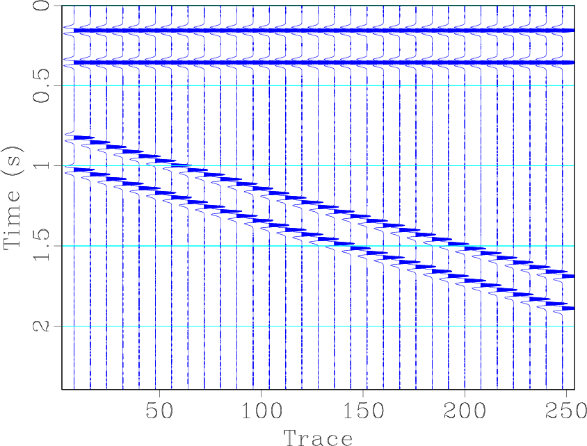
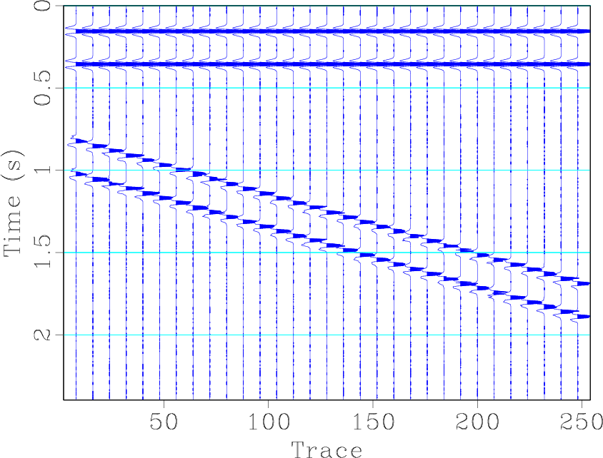
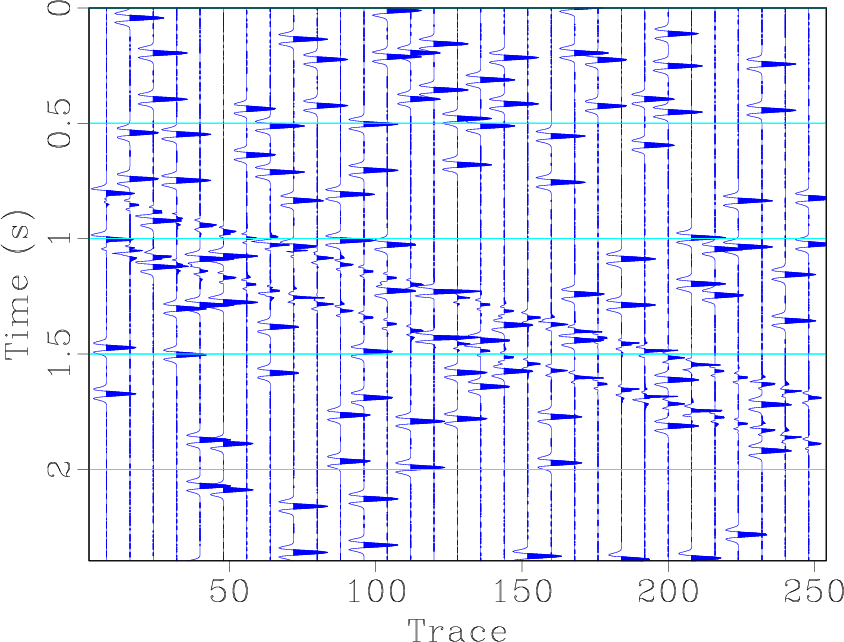
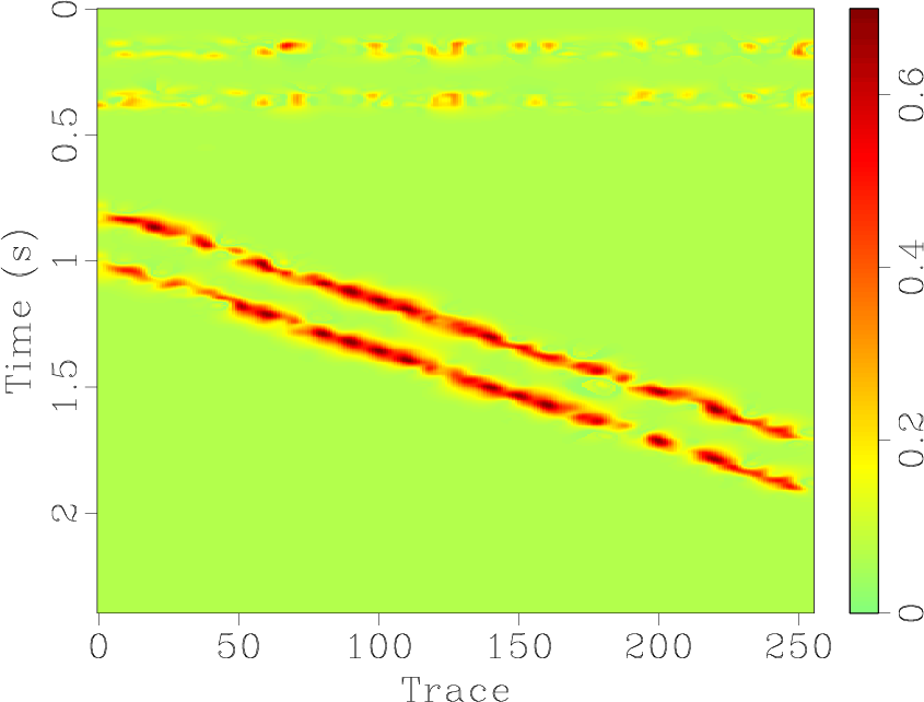
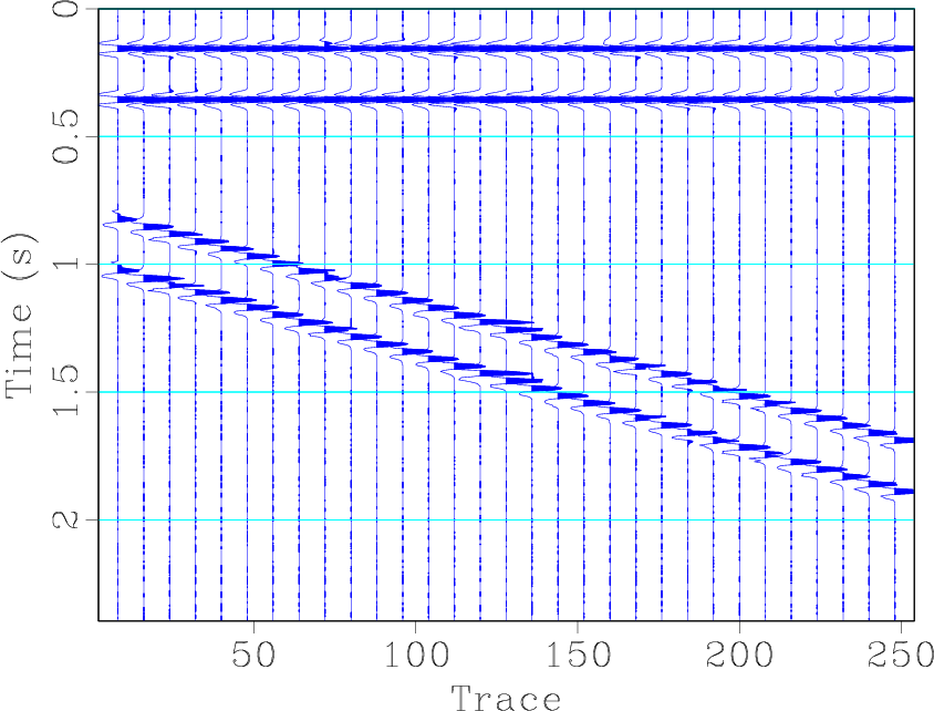
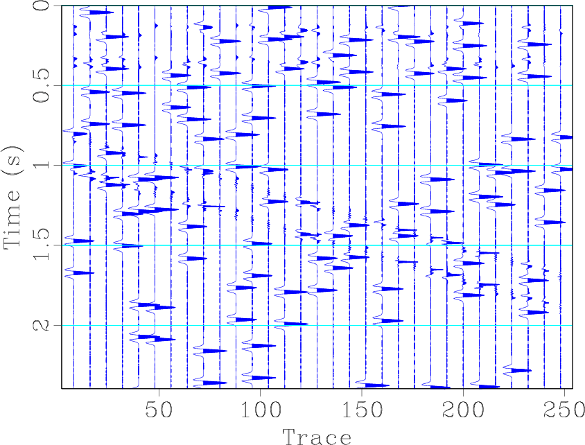
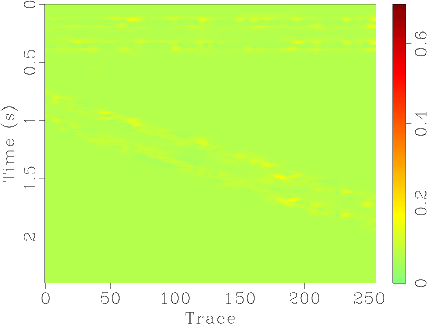
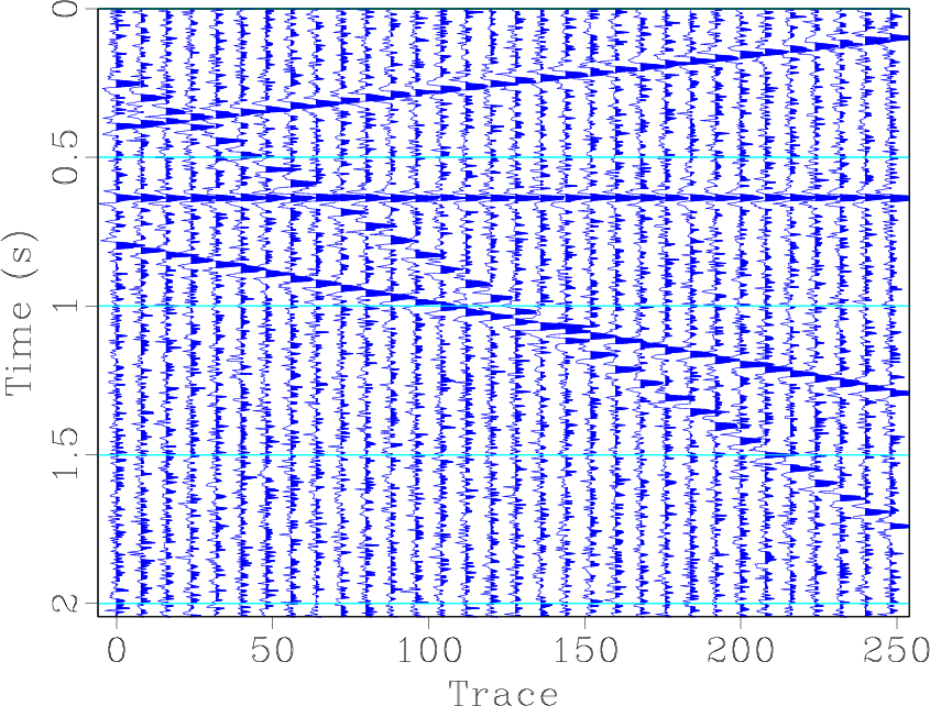
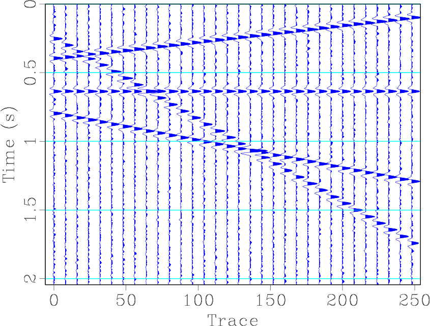
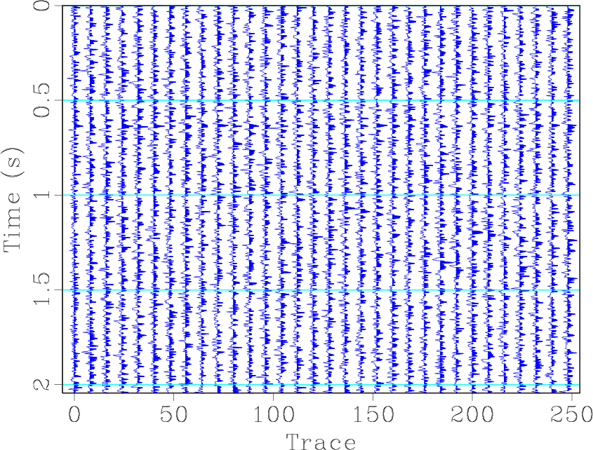
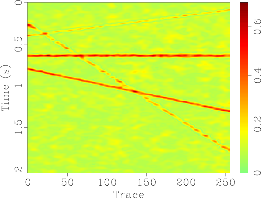
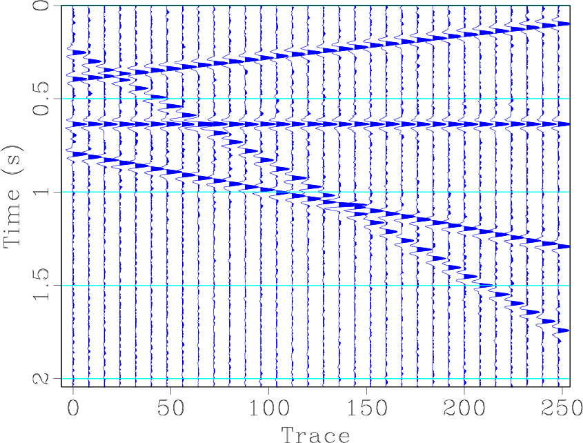
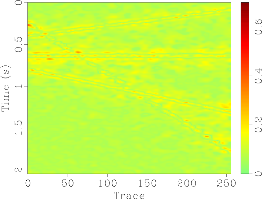
Figure 2. Comparison of using the local-orthogonalization-based random noise attenuation approach for deblending test before and after. (a) Unblended section. (b) Blending noise section. (c) Blended section. (d) Deblended result using MF. (e) Noise section using MF. (f) Local similarity map between (d) and (e). (g) Deblended result using the proposed method. (h) Noise section using the proposed method. (i) Local similarity map between (g) and (h).

In addition to SNR, we also propose to use local similarity (Fomel, 2007a) as a convenient measure to evaluate denoising performance. Appendix B gives a brief review of local similarity. After the local similarity map between the denoised data and removed noise is calculated, we can judge from the local similarity if there is leakage energy in the noise. When the clean data is unknown for field data denoising tests, the SNR based evaluation becomes unavailable. Besides, the SNR is not always the best measurement for denoising performance because it does not measure the signal leakage. However, the local similarity map can always be used to evaluate the denoising performance.

Figure 2 shows the deblending performance using a conventional MF and the proposed denoising approach. The original clean, unblended data are shown in Figure 2a. After blending using a simple random-dithering method (Chen et al., 2014a), we obtained the noisy data containing spike-like blending noise (2c). Figure 2d demonstrates a denoised section after using MF. The noise section corresponding to MF is shown in Figure 2e and contains a certain amount of signal leakage in the form of linear events. Using the proposed denoising approach, we obtained a denoised section with stronger-amplitude linear events. In the corresponding noise section, any coherent linear events are barely noticeable, suggesting a nearly perfect deblending. In this example, because the noise are spike-like blending noise, we did smooth too much during shaping regularization. In this example, the vertical and lateral smoothing radii are both 2 samples. Figures 2f and 2i show local similarity of the noise section to the denoised section before and after using the proposed approach. After applying the proposed method, the noise section exhibits low similarity with the denoised section. Although structure-oriented median filtering can handle the dipping reflector, they can only work well for relative simpler structures where the dip estimation can be precisely obtained, in which case there will be no need to use the proposed approach. However, when the dip estimation is not accurate, or there are conflicting dips in a processing window, the structure-oriented median filtering may not work well, in which case we can use the proposed approach for retrieving the leaked useful energy.

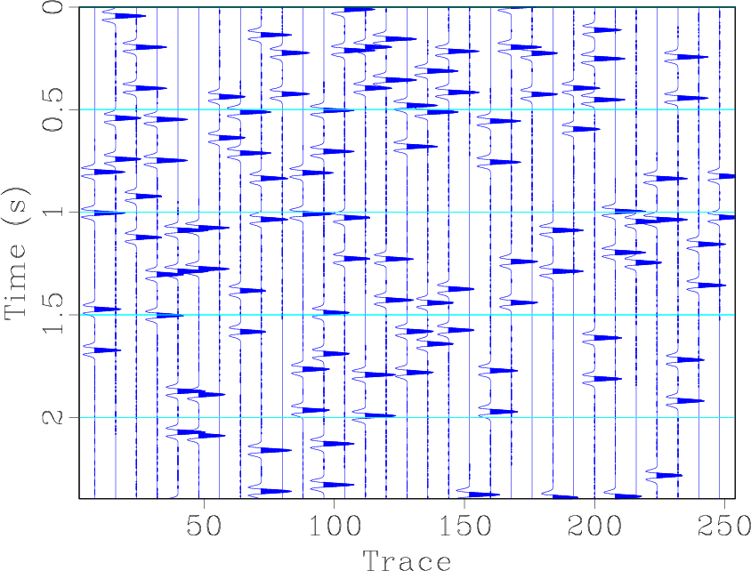
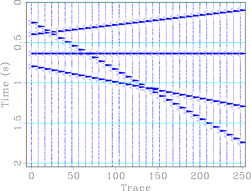
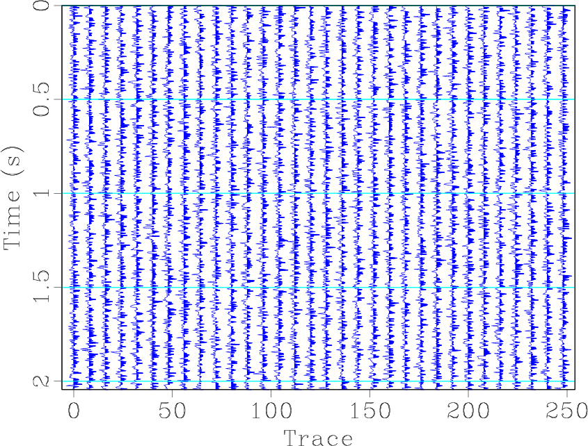
Figure 3 shows the denoising performance based on the conventional $f$ -$x$ deconvolution (Canales, 1984). The clean data is shown in Figure 3a and the noise section, corresponding to $f$ -$x$ deconvolution, is shown in Figure 3f; it contains some horizontal and low-dip-angle signals. The coherent leakage energy is also visible in the local similarity map (Figure 3f). Applying the proposed denoising approach, we obtained a denoised section with stronger-amplitude horizontal events. The corresponding noise section does not contain any coherent signal. In this example, the vertical and lateral smoothing radii are both 25 samples. Figures 3f and 3i denote local similarity of the noise section to the denoised section before and after using the proposed approach. The similarity decreases significantly after applying local orthogonalization.

The SNR comparison before and after using local-orthogonalization approach is summarized in Table 1.

Test	Deblending	denoising
Original (dB)	1.173	-1.72
Initially denoised (dB)	17.65	21.21
Orthogonalized (dB)	20.95	25.30

Table 1. Comparison of SNR before and after using the proposed approach.

c,n,cn,cfx,cdifffx,csimi-difffx,cfx2,cdifffx2,csimi-difffx2
Figure 3. Comparison of using the local-orthogonalization-based random noise attenuation approach for denoising test before and after. (a) Clean section. (b) Random noise section. (c) Noisy section. (d) Denoised result using $f$ -$x$ deconvolution. (e) Noise section using $f$ -$x$ deconvolution. (f) Local similarity map between (d) and (e). (g) Denoised result using the proposed method. (h) Noise section using the proposed method. (i) Local similarity map between (g) and (h).

Random noise attenuation using local signal-and-noise orthogonalization