|
|
|
|
A reversible transform for seismic data processing |
|
|---|
|
data
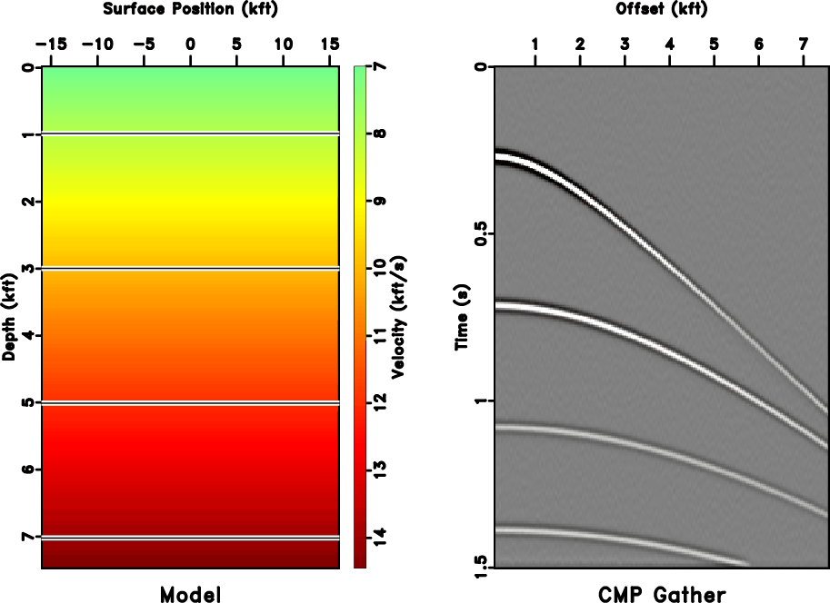
Figure 2. Synthetic CMP gather. Left: Velocity model. Four reflectors are placed in a background velocity that increases linearly with depth ( |
|
|

|
|---|
|
nmomat
Figure 3. The forward NMO transform matrix can be composed as the Hadamard (entry-wise) product of the inverse Fourier transform matrix (left) and the NMO forward shifting matrix for an example trace at |
|
|

|
|---|
|
inmomat
Figure 4. The inverse NMO transform matrix can be composed as the Hadamard product of the forward Fourier transform matrix (left) and the NMO reverse shifting matrix for an example trace at |
|
|

|
|---|
|
nmo
Figure 5. Reversible NMO applied to gather from Figure 2. Left: Semblance panel and picked velocity. Center: NMO-corrected gather. Right: Inverse NMO applied to gather. |
|
|

|
|---|
|
stretch
Figure 6. NMO applied to and removed from a single trace at |
|
|
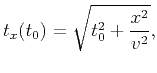
The kinematics of the shift required for the NMO correction simply shift data values backwards from input time, ![]() , to output time,
, to output time, ![]() , where
, where ![]() depends on
depends on ![]() . For ideal continuous data, the input and output times are both arbitrary, but for discrete field data, both must coincide exactly with a sampling time or values must be interpolated.
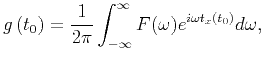
In the continuous case, this is exactly a nonstationary shift by combination as described by Margrave (1998), where for the NMO correction, the nonstationary shift is expressed as,
. For ideal continuous data, the input and output times are both arbitrary, but for discrete field data, both must coincide exactly with a sampling time or values must be interpolated.
In the continuous case, this is exactly a nonstationary shift by combination as described by Margrave (1998), where for the NMO correction, the nonstationary shift is expressed as,
In the case of the NMO correction, the time distortion caused by the shift is well-known, and referred to as NMO stretch (Buchholtz, 1972; Dunkin and Levin, 1973).
Various authors have developed strategies for handling the effects of NMO stretch in practical seismic data processing (Perroud and Tygel, 2004; Shatilo and Aminzadeh, 2000; Miller, 1992).
NMO stretch manifests the most at far offsets and early times, where the NMO correction is the most severe.
The waveform of an event in this area is stretched to a longer period as the NMO correction is applied (Yilmaz, 2001).
The amplitude of that event is not affected, but its time distortion causes an alteration in its frequency content.
Specifically, the lower frequency content is boosted, and since the amplitude of the waveform is maintained, a nonphysical addition of energy to the input signal has occurred.
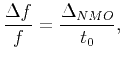
Yilmaz (2001) quantifies the frequency distortion caused by NMO stretch in terms of
![]() and
and ![]() :
:
where, f is the dominant frequency of the input waveform. This expression is derived from geometric arguments and assumes
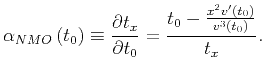
![]() (Yilmaz, 2001). Another approach to describing NMO stretch comes from analyzing the effects of the NMO correction in terms of instantaneous frequency (Barnes, 1992). This approach provides excellent insight into the frequency distortion, and yields an exact expression for NMO stretch,
(Yilmaz, 2001). Another approach to describing NMO stretch comes from analyzing the effects of the NMO correction in terms of instantaneous frequency (Barnes, 1992). This approach provides excellent insight into the frequency distortion, and yields an exact expression for NMO stretch, ![]() :
:
where ![]() is the derivative of v with respect to time (Barnes, 1992). This expression quantifies NMO stretch without approximations, and is not dependent only on the dominant frequency as in equation 23. It is valid for variable velocity models, and for a constant velocity model, the derivative of velocity goes to zero, and
is the derivative of v with respect to time (Barnes, 1992). This expression quantifies NMO stretch without approximations, and is not dependent only on the dominant frequency as in equation 23. It is valid for variable velocity models, and for a constant velocity model, the derivative of velocity goes to zero, and ![]() agrees with the approximation in equation 23.
agrees with the approximation in equation 23.
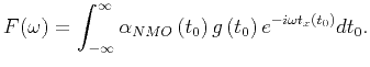
As equation 24 suggests, NMO stretch is itself nonstationary, and therefore cannot be removed exactly using stationary filtering theory. However, since the data processing transform takes advantage of nonstationary filtering, NMO stretch can be removed exactly. Substituting the NMO variables,
![]() and
and
![]() into 11, gives the inverse NMO transform:
into 11, gives the inverse NMO transform:
The inverse NMO transform does account for NMO stretch, and in fact,
![]() exactly. Realizing that the two are equivalent leads to a straightforward (once nonstationary filtering is allowed) perspective on predicting and quantifying NMO stretch. Further, Barnes (1992) proves, in terms of instantaneous power and energy spectra, that
exactly. Realizing that the two are equivalent leads to a straightforward (once nonstationary filtering is allowed) perspective on predicting and quantifying NMO stretch. Further, Barnes (1992) proves, in terms of instantaneous power and energy spectra, that ![]() , and therefore
, and therefore
![]() indeed describe the nonphysical energy change caused by the NMO correction.
Figure 6 shows the application and removal of the NMO correction to a single trace.
Two cases are shown for inverse NMO: one where
indeed describe the nonphysical energy change caused by the NMO correction.
Figure 6 shows the application and removal of the NMO correction to a single trace.
Two cases are shown for inverse NMO: one where ![]() is not included and one where it is.
In the case where
is not included and one where it is.
In the case where ![]() is used, the amplitude is recovered correctly, whereas when
is used, the amplitude is recovered correctly, whereas when ![]() is not used, inverse NMO preserves the energy of the NMO-corrected trace, leading to too much energy in the recovered signal.
It can be shown that
is not used, inverse NMO preserves the energy of the NMO-corrected trace, leading to too much energy in the recovered signal.
It can be shown that ![]() plays a similar role in accounting for nonphysical energy changes introduced by other imaging steps such as so-called ``Stolt stretch'' associated with Stolt migration (Burnett and Ferguson, 2008b).
plays a similar role in accounting for nonphysical energy changes introduced by other imaging steps such as so-called ``Stolt stretch'' associated with Stolt migration (Burnett and Ferguson, 2008b).
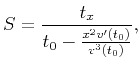
The NMO transform acts as a map between the uncorrected spectrum and the NMO-corrected trace. As such, the first step in implementing the forward NMO transform on a trace is to apply a standard forward Fourier transform to the input trace. This gives the uncorrected spectrum, which becomes the input column vector for a matrix vector multiplication. Following 16, the discrete NMO transform is given as,
One can also decompose the forward NMO transform operator as the Hadamard product of the inverse Fourier transform matrix and the NMO shifting matrix following 18 (see Figure 3). The frequency axis of the shifting operator must exactly match the frequency axis used for the forward Fourier transform, since it will simultaneously remove that Fourier transform as it NMO-corrects the data. The inverse NMO transform can also be implemented by matrix-vector multiplication by substituting ![]() and
and
![]() into 17. As seen in Figure 4, the full inverse NMO transform operator can be decomposed as the Hadamard product of the forward Fourier transform matrix and the NMO reverse shifting matrix.
We conclude this example by removing the NMO correction by transform, shown in Figure 5.
Most of the gather is recovered nearly perfectly-only parts which were mapped to
into 17. As seen in Figure 4, the full inverse NMO transform operator can be decomposed as the Hadamard product of the forward Fourier transform matrix and the NMO reverse shifting matrix.
We conclude this example by removing the NMO correction by transform, shown in Figure 5.
Most of the gather is recovered nearly perfectly-only parts which were mapped to ![]() are not recovered well.
are not recovered well.
|
|
|
|
A reversible transform for seismic data processing |
![$\displaystyle g \left( \left[ t_{0}\right] _j \right) = \sum _{l=1}^N \frac{e^{i \, \omega_l p \left( t_{0,j} \right)}}{2 \, \pi} \, F \left( \omega_l \right).$](img94.png)