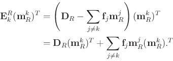
Although K-SVD can obtain very successful performance in a number of sparse representation based approaches, since there involves many SVD operations in the K-SVD algorithm, it is very computationally expensive. Especially when utilized in multidimensional seismic data processing (e.g. 3D or 5D processing), the computational cost is not tolerable. The sequential generalized K-means algorithm (SGK) was proposed to increase the computational efficiency (Sahoo and Makur, 2013). SGK tries to solve slightly different iterative optimization problem in sparse coding as equation 3:
 |
(8) |
 indicates that
 has all 0s except 1 in the th position. The dictionary updating in SGK algorithm is also different.
In SGK, equation 6 also holds. Instead of using SVD to minimize the objective function, which is computationally expensive, SGK turns to use least-squares method to solve the minimization problem. Taking the derivative of
has all 0s except 1 in the th position. The dictionary updating in SGK algorithm is also different.
In SGK, equation 6 also holds. Instead of using SVD to minimize the objective function, which is computationally expensive, SGK turns to use least-squares method to solve the minimization problem. Taking the derivative of
 with respect to
 and setting the result to 0 gives the following equation:
 |
(9) |
solving equation 9 leads to
 |
(10) |
It can be derived further that
 |
(11) |
Here,
 has the same meaning as
 shown in equation 5 except for a smaller size due to the selection set
  that selects the entries in
 that are non-zero.
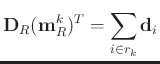
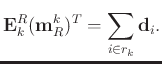
Since
 , as constrained in equation 8 then
 |
(12) |
Since
 is a smaller version of row vector
and all its entries are all equal to 1,
is a smaller version of row vector
and all its entries are all equal to 1,
 is simply a summation over all the column vectors in
. Considering that
is simply a summation over all the column vectors in
. Considering that
 ,
,
 |
(13) |
Following equation 13, equation 11 becomes
 |
(14) |
It is simple to derive that
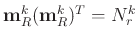 , where
  denotes the number of elements in the set , or the number of training signals associated with the atom
. The
denotes the number of elements in the set , or the number of training signals associated with the atom
. The  th atom in
 is
is
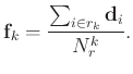 |
(15) |
Thus, in SGK, one can avoid the use of SVD. Instead the trained dictionary can be simply expressed as an average of several training signals. In this way, SGK can obtain significantly higher efficiency than K-SVD. In the next section, I will use several examples to show that the overall denoising performance does not degrade when one can obtain a much faster implementation.
2020-04-03