|
|
|
|
Stacking seismic data using local correlation |
The problem of combining a collection of seismic traces into a
single trace is commonly referred to as stacking in seismic data processing.
This process is used to attenuate random noise and simultaneously
amplify the coherent signal in the gather. Typically, the desired
stacked trace is estimated by averaging traces from the CMP
gather (Mayne, 1962):
For using time-dependent smooth weights in the stacking process, we choose the local correlation coefficient from the previous section as weights to stack seismic data. We find that local correlation better characterizes local similarity between prestack and reference traces than the sliding-window method.
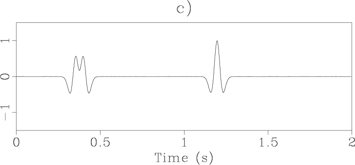
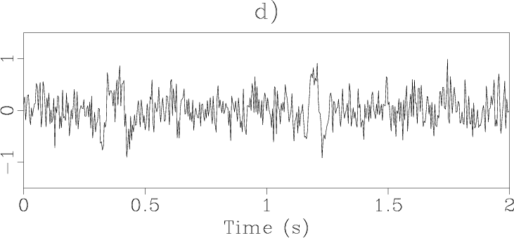
Consider the two noisy signals with Gaussian random noise but different noise
levels in Figure 1c and
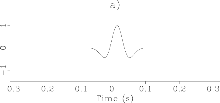
1d. The signals are derived from
adding noise on convolution of the Ricker wavelet (Figure
1a)
with synthetic reflectivity
(Figure 1b). The distribution of
noise in
(Figure 1c) is
![]() , where
, where ![]() and
and ![]() are mean and variance of noise, respectively. The distribution of noise in
(Figure 1d) is
are mean and variance of noise, respectively. The distribution of noise in
(Figure 1d) is
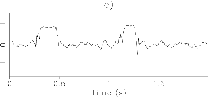
![]() . The sliding-window
correlation and local correlation
between Figure 1c and
Figure 1d are shown in
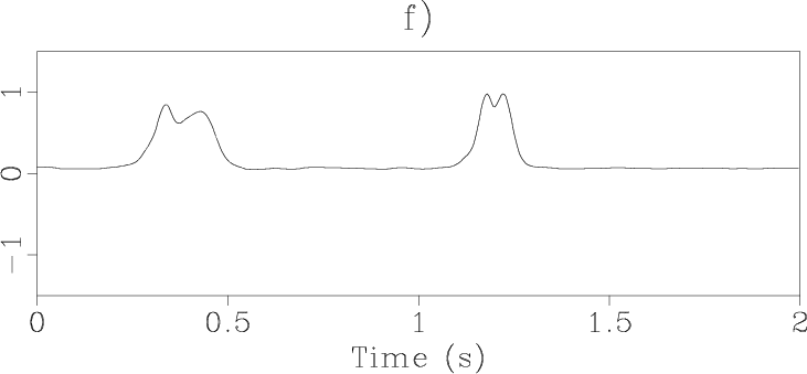
Figure 1e and
Figure 1f, respectively.
Note that local correlation coefficients
(Figure 1f) are smooth and
better distinguish the thin layer, represented by the first two reflectivities
in Figure 1b. In application to
stacking, the prestack trace is
analogous to Figure 1d with
larger variance noise, and the reference trace is analogous to
Figure 1c with smaller variance
noise.
. The sliding-window
correlation and local correlation
between Figure 1c and
Figure 1d are shown in
Figure 1e and
Figure 1f, respectively.
Note that local correlation coefficients
(Figure 1f) are smooth and
better distinguish the thin layer, represented by the first two reflectivities
in Figure 1b. In application to
stacking, the prestack trace is
analogous to Figure 1d with
larger variance noise, and the reference trace is analogous to
Figure 1c with smaller variance
noise.

|
|---|
|
ricker,ref,signal1,signal2,wcorr,simi
Figure 1. (a) Zero-phase Ricker wavelet. (b) Reflection coefficient. (c) Noisy signal with |
|
|
To implement seismic data stacking using local correlation, we
first apply the equal-weight stack to the NMO-corrected CMP gather
to obtain the reference trace. Then we compute the local correlation
coefficients between the reference trace and the NMO-corrected
CMP gather and apply soft thresholding (Donoho, 1995) to all local
correlation coefficients. Finally, we apply the weighted stack to the
CMP gather using local correlation to get the final stacked trace.
Mathematically, stacking using the local correlation approach
modifies equation 9 to
 is the sum of weights of the
 Changes occurring between equation 9 and equations 10 and 11 result from time-dependent smooth weights for the stack and application of thresholding to the weights. All local correlation coefficients below a specified threshold are discarded, and the rest, with values above the threshold, are included. We thus stack only those parts of prestack data whose similarity to the reference trace is comparatively large. Equations 10 and 11 implicitly estimate the noise variance by analyzing local cross-correlations between prestack trace and the reference trace. This operation can be understood as a nonlinear filter that enhances the coherency of events. We perform this operation for all gathers using this method to improve the stack profile.
When applied after angle-domain migration, normalization provided by soft thresholding is analogous to true-amplitude illumination compensation from the so-called Beylkin determinant (Audebert and Froidevaux, 2005; Albertin et al., 1999). Local correlation normalizes the image by the number of strongly illuminated angles in angle-domain CIGs.
In the following, we discuss the distinctions between seismic stacking using local correlation and other methods. Our method creates time-dependent smooth weights without depending on sliding windows, as compared to other weighted stacking methods such as statistically optimal stacking (Neelamani et al., 2006; Robinson, 1970) and the semblance method (Yilmaz, 2001). In contrast to smart stacking, proposed by (Rashed, 2008) and based on sign difference between sample point and the alpha-trimmed mean to remove frequency distortions, our method applies waveform similarity between prestack trace and mean to make the stacking selective.
|
|
|
|
Stacking seismic data using local correlation |