|
|
|
|
Deblending using a space-varying median filter |


|
|---|
|
data-csg,data-b,datas-csg,data-b-svmf-cmg,data-b-svmf-csg,data-b-svmf-cog
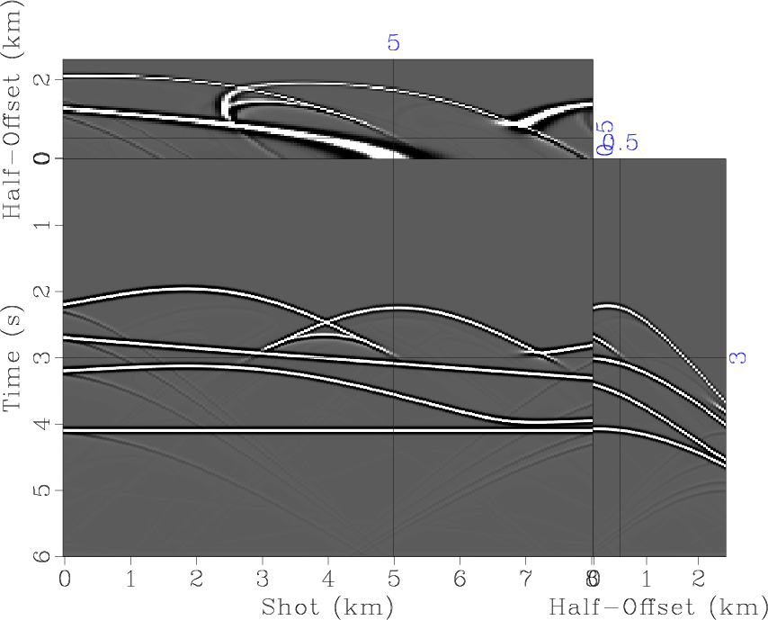
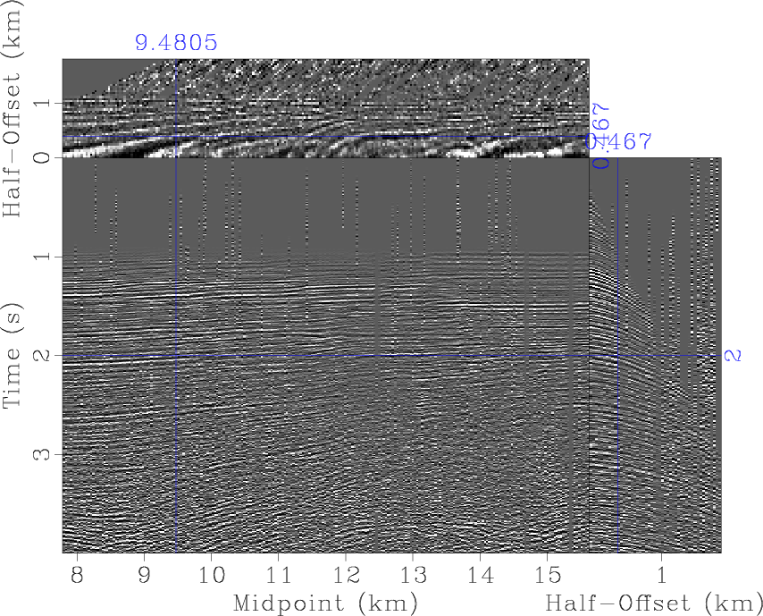
Figure 10. (a) Synthetic data in TSO domain. (b) Blended data in TMO domain. (c) Blended data in TSO domain. (d) Deblended data by applying SVMF in CMG. (e) Deblended data in TSO domain corresponding to (d). (f) Deblended data by applying SVMF in COG. |
|
|
|
|---|
|
data-b-svmf-cmg-zoom,data-b-svmf-cog-zoom
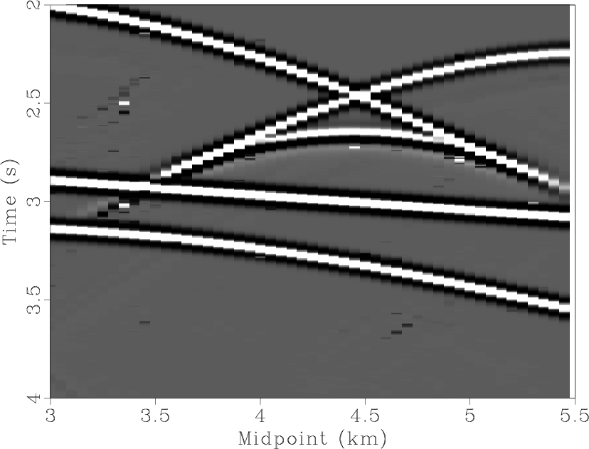
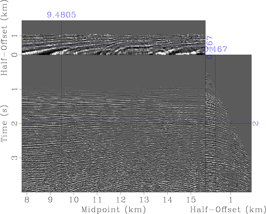
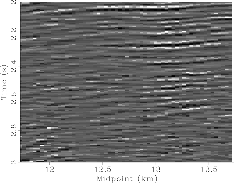
Figure 11. Zoomed COG (time: 2 s -4 s, midpoint: 3.0 km - 5.5 km, half-offset: 0.5 km). (a) Applying SVMF in CMG (from Figure 10d). (b) Applying SVMF in COG (from Figure 10f). |
|
|
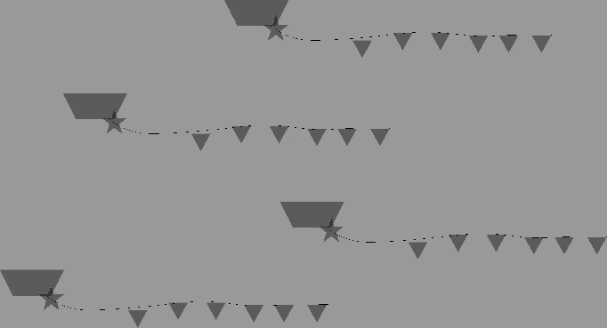
The third example is a synthetic prestack time-shot-offset (TSO) domain data cube (Figure 10). There are 1501 time samples in this synthetic example and the temporal sampling is 4 ms. The peak frequency is 10 Hz. There are 251 shots and 51 receivers in this example. The shot and receiver intervals are both 50 m. I blended the data by simulating a independent marine-streamer simultaneous shooting (IMSSS) acquisition with two sources. The demonstration of the IMSSS is shown in Figure 14. Note that the number of simultaneous sources need not be limited to four. The shooting vessels shoot independently as in the conventional way and obtain their own data. With ![]() sources, the efficiency can be increased by
sources, the efficiency can be increased by ![]() times. The increased efficiency, however, is compromised by interference among different sources. The unblended and blended data are shown in Figures 10a and 10c, respectively. Figure 10c shows that the blending interference turns to be coherent in common-shot gather (CSG). After transforming the data from CSG to common-midpoint gather (CMG), the interference turns to be incoherent spike-like noise. I applied SVMF to both CMG and common-offset gather (COG) in the TMO domain; the results are shown in Figures 10d and 10e, respectively. In order to maximize the effectiveness of SVMF, I applied a normal move-out (NMO) with an approximate velocity in CMG, in order to make the events flatter. However, this strategy was not feasible in COG. Thus, filtering in CMG will preserve more useful signal than filtering in COG. Figure 11 shows a comparison between two zoomed COG from Figures 10d and 10f, respectively. The comparison confirm the fact that applying SVMF in CMG will preserve more more useful signal that applying SVMF in COG. Figure 10e shows the deblended data in the TSO domain by filtering in CMG. Comparing the deblended data show in Figure 10e with blended data shown in Figure 10c, it is clear that the deblending has been successful. The initial filter length involved in SVMF for this example is chosen as 7. The increments/decrements
times. The increased efficiency, however, is compromised by interference among different sources. The unblended and blended data are shown in Figures 10a and 10c, respectively. Figure 10c shows that the blending interference turns to be coherent in common-shot gather (CSG). After transforming the data from CSG to common-midpoint gather (CMG), the interference turns to be incoherent spike-like noise. I applied SVMF to both CMG and common-offset gather (COG) in the TMO domain; the results are shown in Figures 10d and 10e, respectively. In order to maximize the effectiveness of SVMF, I applied a normal move-out (NMO) with an approximate velocity in CMG, in order to make the events flatter. However, this strategy was not feasible in COG. Thus, filtering in CMG will preserve more useful signal than filtering in COG. Figure 11 shows a comparison between two zoomed COG from Figures 10d and 10f, respectively. The comparison confirm the fact that applying SVMF in CMG will preserve more more useful signal that applying SVMF in COG. Figure 10e shows the deblended data in the TSO domain by filtering in CMG. Comparing the deblended data show in Figure 10e with blended data shown in Figure 10c, it is clear that the deblending has been successful. The initial filter length involved in SVMF for this example is chosen as 7. The increments/decrements ![]() are chosen as the default values.
are chosen as the default values.


|
|---|
|
gulf-csg,gulf-b,gulfs-csg,gulf-b-svmf-cmg,gulf-b-svmf-csg,gulf-b-svmf-cog
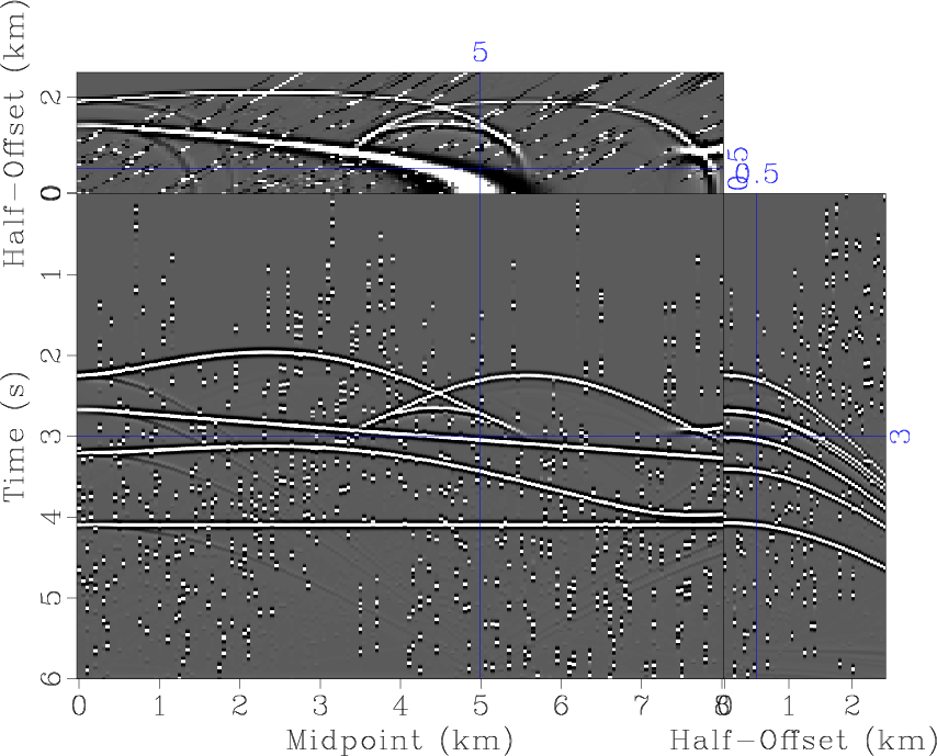
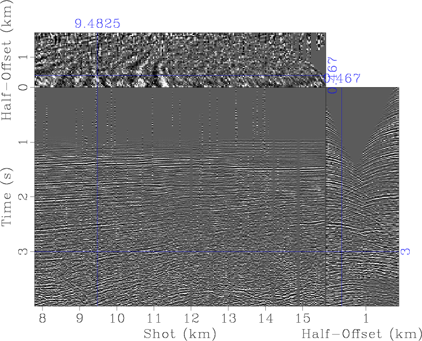
Figure 12. (a) Marine field data in TSO domain. (b) Blended data in TMO domain. (c) Blended data in TSO domain. (d) Deblended data by applying SVMF in CMG. (e) Deblended data in TSO domain corresponding to (d). (f) Deblended data by applying SVMF in COG. |
|
|
|
|---|
|
gulf-b-svmf-cmg-zoom,gulf-b-svmf-cog-zoom
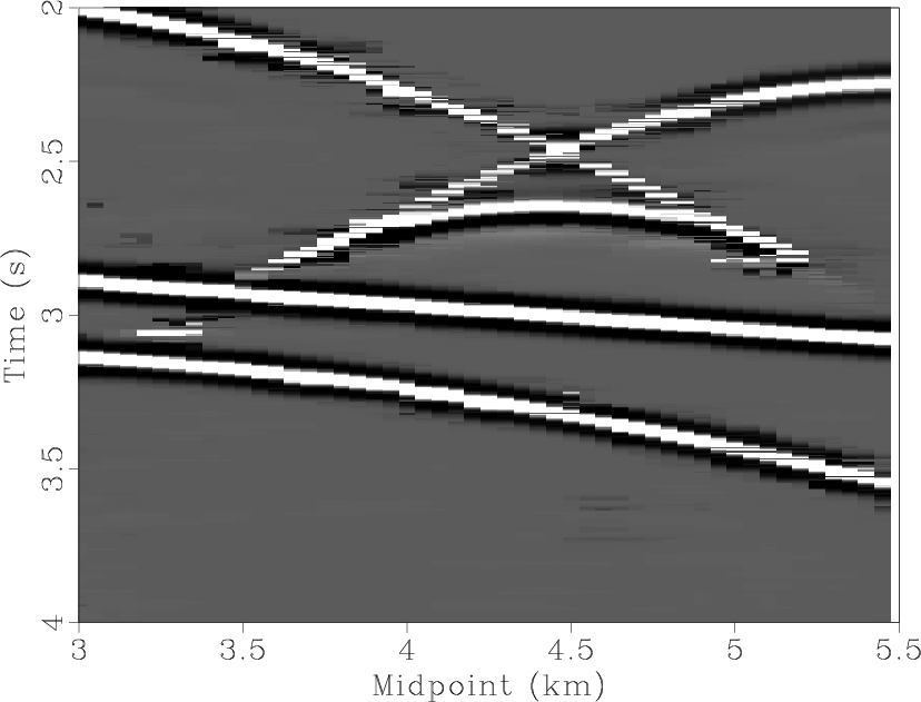
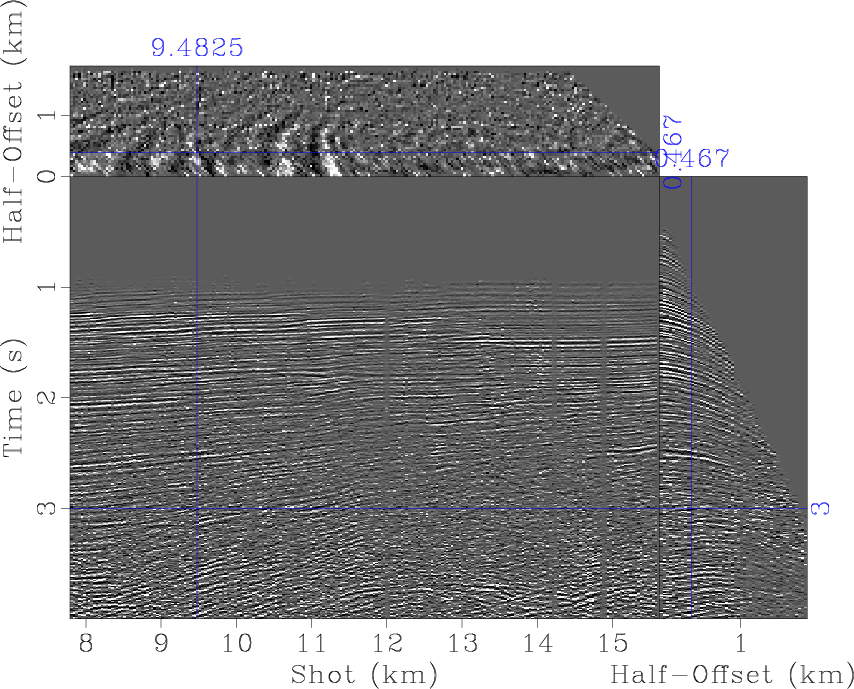
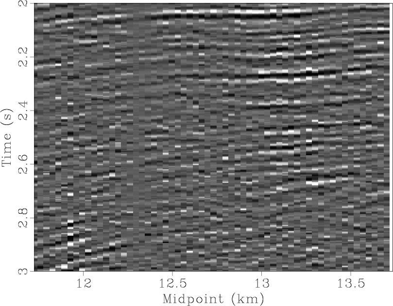
Figure 13. Zoomed COG (time: 2 ms - 3 ms, midpoint: 11.725 km - 13.735 km, half-offset: 0.635 km). (a) Applying SVMF in CMG (from Figure 12d). (b) Applying SVMF in COG (from Figure 12f). |
|
|
The fourth example is a field prestack time-shot-offset (TSO) domain data cube (Figure 12). There are 1000 time samples in this synthetic example and the temporal sampling is 4 ms. There are 291 shots and 48 receivers in this example. The shot and receiver intervals are both 33.5 m. The blended acquisition is the same as the third example. In this case, the blending noise in CMG turns to be string-like noise. However, the string-like noise appears as spike-like noise along spatial direction. Thus, we can still use the proposed SVMF to remove the blending noise. The unblended data, blended data, deblended data in different domains are all shown in Figure 12. The layout of different figures is exactly the same as the third example. Figure 13 shows the comparison between two zoomed COG corresponding to different filtering gathers. Figure 13a preserves more small features compared with Figure 13a, confirming the fact that the proposed approximate NMO can help preserve more useful energy. Comparing the deblended data show in Figure 12e with blended data shown in Figure 12c, it is clear that the deblending for the field data example is also successful. The initial filter length involved in SVMF for this example is chosen as 5 to be more conservative. The increments/decrements ![]() are chosen as the default values.
are chosen as the default values.
|
|---|
|
streamer-demo
Figure 14. Demonstration of independent marine-streamer simultaneous shooting (IMSSS) acquisition with four sources. |
|
|
|
|
|
|
Deblending using a space-varying median filter |