|
|
|
|
A variational approach for picking optimal surfaces from semblance-like panels |


|
|---|
|
gom-cmps-0,gom-vscan-0
Figure 7. (a) CMP gathers from a Gulf of Mexico field data set; (b) NMO velocity scan for the CMP gathers in Figure 7a. |
|
|


|
|---|
|
gom-plotmod-0,gom-plotmod-1,gom-plotmod-2,gom-plotmod-3,gom-plotmod-4,gom-plotmod-5,gom-plotmod-6,gom-plotmod-7,gom-plotmod-8
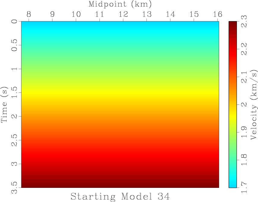
Figure 8. Random selection of nine constant-gradient velocity models from the 125 used as starting models. |
|
|
To illustrate how the continuation approach reduces the dependence of the final model on the starting model, we generate 125 constant-gradient velocity models which are clipped to the range of the velocity scan. A random selection of nine of these is shown in Figures 8a through 8i. These 125 starting models are used with the continuation picking approach over the ten smoothness levels and their cost convergence, or model cost by iteration according to Equation 4 as measured on the least-smoothed semblance volume in Figure 7b, is plotted in Figure 9a. If convergence is achieved before the maximum possible number of iterations, the final cost is repeated in these plots through the maximum iteration number. The lowest cost achieved is plotted as a dashed black line in that plot. For comparison, we also use the collection as starting models for iterative picking on the least smooth
![]() without continuation. That cost convergence is plotted in Figure 9b. Again, the lowest cost achieved by the continuation picking approach is plotted as a dashed black line and, if convergence is achieved before the maximum possible number of iterations, the final cost is repeated in these plots through the maximum iteration number.
without continuation. That cost convergence is plotted in Figure 9b. Again, the lowest cost achieved by the continuation picking approach is plotted as a dashed black line and, if convergence is achieved before the maximum possible number of iterations, the final cost is repeated in these plots through the maximum iteration number.


|
|---|
|
gom-costs,gom-noncont-costs
Figure 9. Cost convergence |
|
|


|
|---|
|
gom-best-model-final-plot,gom-worst-model-final-plot,gom-nocont-best-model-final-plot,gom-nocont-worst-model-final-plot
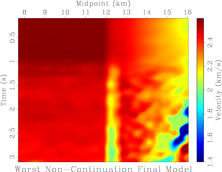
Figure 10. Lowest and highest cost final models from velocity picking using the 125 constant-gradient starting models: (a) lowest cost continuation final model; (b) highest cost continuation final model; (c) lowest cost non-continuation final model; (d) highest cost non-continuation final model. |
|
|
The final continuation model with the lowest cost (
![]() ) is plotted in Figure 10a, and the continuation model with the highest cost (
) is plotted in Figure 10a, and the continuation model with the highest cost (
![]() ) is shown in Figure 10b. The lowest cost (
) is shown in Figure 10b. The lowest cost (
![]() ) non-continuation final model can be seen in Figure 10c, and the highest cost (
) non-continuation final model can be seen in Figure 10c, and the highest cost (
![]() ) non-continuation final model is displayed in Figure 10d. To show how the continuation approach tends to produce similar final models, we compute the
) non-continuation final model is displayed in Figure 10d. To show how the continuation approach tends to produce similar final models, we compute the ![]() difference between the lowest cost continuation final model shown in Figure 10a and every update for every continuation model update and plot them in
difference between the lowest cost continuation final model shown in Figure 10a and every update for every continuation model update and plot them in ![]() scale in Figure 11a. If convergence is achieved before the maximum possible number of iterations, the final
scale in Figure 11a. If convergence is achieved before the maximum possible number of iterations, the final ![]() misfit is repeated in these plots thru the maximum iteration number. The
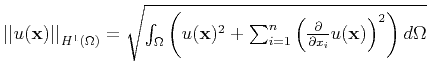
misfit is repeated in these plots thru the maximum iteration number. The ![]() norm of a function
norm of a function
![]() ,
,
![]() is defined as
is defined as
 , and the
 ![]() difference or misfit of two functions
difference or misfit of two functions
![]() is
is
![]() . This norm is used because it is the norm of the Hilbert space where minimizing surfaces of Equation 4 exist, and the norm in which convergence to minimizers should occur. The mean
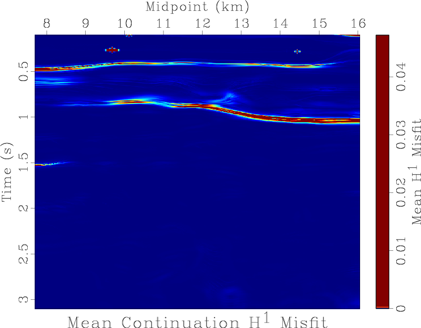
. This norm is used because it is the norm of the Hilbert space where minimizing surfaces of Equation 4 exist, and the norm in which convergence to minimizers should occur. The mean ![]() difference between the lowest-cost continuation final model and each of the 125 continuation final models is displayed in Figure 11b. These visualizations are also generated for
difference between the lowest-cost continuation final model and each of the 125 continuation final models is displayed in Figure 11b. These visualizations are also generated for ![]() scale misfit between the lowest-cost continuation final model and each non-continuation update, as shown in Figure 11c, and the mean
scale misfit between the lowest-cost continuation final model and each non-continuation update, as shown in Figure 11c, and the mean ![]() misfit between non-continuation final models and the lowest-cost continuation final model in Figure 11d. Notice that in the continuation
misfit between non-continuation final models and the lowest-cost continuation final model in Figure 11d. Notice that in the continuation ![]() convergence plot shown in Figure 11a, the lowest-cost model can be seen in red descending to an isolated end point around -11 near iteration 145. This is because, in the next iteration, it achieves the lowest cost final model, and thus the
convergence plot shown in Figure 11a, the lowest-cost model can be seen in red descending to an isolated end point around -11 near iteration 145. This is because, in the next iteration, it achieves the lowest cost final model, and thus the ![]() misfit is zero, the log of which is undefined.
misfit is zero, the log of which is undefined.


|
|---|
|
gom-convergence,gom-models-h1mis,gom-nocont-convergence,gom-nocont-models-h1mis
Figure 11. (a) |
|
|
The lowest cost continuation velocity model, which is subsequently referred to as the ``best model,'' is used for seismic processing of this data set. The left panel of Figure 12 visualizes the best model overlaid on the semblance scan for a CMP gather at 8.5 km. The right panel illustrates that gather after NMO correction with the best model has been applied. Figure 13a contains stacked data following NMO correction using the best model. Diffraction data are extracted from that stack by using plane-wave destruction filters (Fomel, 2002; Decker et al., 2013; Fomel et al., 2007) to predict reflection signal and remove it from zero-offset data, leaving the set of diffractions and noise, which is displayed in Figure 13b. The best model is used for Kirchhoff time migration on the NMO stack data, whose image is shown in Figure 14a, and on the diffraction data to create the diffraction image in Figure 14b.

|
|---|
|
gom-gather-0
Figure 12. Illustration of the effects of the picking algorithm on a CMP centered at 8.5 km. Left panel contains a semblance scan for the CMP gather centered here overlaid by lowest cost final continuation velocity model from Figure 10a in solid fuchsia. Right panel contains the NMO corrected gather using that lowest cost final velocity model. |
|
|


|
|---|
|
gom-best-model-nmo-stk,gom-best-model-nmo-stk-difr
Figure 13. (a) NMO corrected stack generated using the lowest cost continuation model shown in Figure 10a; (b) Diffraction data extracted from the NMO stack in Figure 13a using plane-wave destruction filters. |
|
|


|
|---|
|
gom-best-model-image,gom-best-model-difr-img
Figure 14. Kirchhoff time images generated using the lowest cost continuation model shown in Figure 10a corresponding to (a) the complete NMO stack data displayed in Figure 13a; (b) the diffraction data shown in Figure 13b. |
|
|
The continuation approach to picking velocities is able to overcome local minima and generate final models of similar cost and appearance relative to those created without continuation. As can be seen in the cost convergence plots for the continuation approach, Figure 9a, and the cost convergence plot without continuation, Figure 9b, the continuation approach leads to uniformly low-cost models relative to the approach without continuation. Indeed, the lowest-cost model achieved with continuation possesses a cost of
![]() while the highest cost model possesses a cost of
while the highest cost model possesses a cost of
![]() . These costs are significantly lower than the starting model costs for the 125 constant-gradient models, which range from roughly
. These costs are significantly lower than the starting model costs for the 125 constant-gradient models, which range from roughly
![]() to
to
![]() . Examining Figure 9a, none of the final models from the 125 has a final cost that is visibly different from the lowest-cost model. Comparing this result to those of cost convergence without continuation, shown in Figure 9b, the lowest-cost non-continuation model has a higher cost (
. Examining Figure 9a, none of the final models from the 125 has a final cost that is visibly different from the lowest-cost model. Comparing this result to those of cost convergence without continuation, shown in Figure 9b, the lowest-cost non-continuation model has a higher cost (
![]() ) than the highest-cost continuation model. There is also a significantly larger spread in final costs.
) than the highest-cost continuation model. There is also a significantly larger spread in final costs.
The continuation approach tends to generate to models that appear similar. The lowest-cost continuation model, plotted in Figure 10a, and the highest-cost continuation model in Figure 10b are visibly the same. Areas where the continuation models tend to differ can be seen in the mean continuation final model ![]() misfit plot of Figure 11b. This appears to be primarily confined to two approximately horizontal features near 0.5 and 1 s, which coincide with areas where velocity changes rapidly in the lowest-cost continuation final model, Figure 10a. The lowest-cost non-continuation model in Figure 10c has a reasonably similar appearance to the lowest-cost continuation final model, although it possesses some anomalous ``blobs'' that are not geologically plausible. The highest-cost non-continuation final model in Figure 10d bears little, if any, resemblance to the lowest-cost continuation final model, and does not appear particularly geological or informative of the subsurface. Mean
misfit plot of Figure 11b. This appears to be primarily confined to two approximately horizontal features near 0.5 and 1 s, which coincide with areas where velocity changes rapidly in the lowest-cost continuation final model, Figure 10a. The lowest-cost non-continuation model in Figure 10c has a reasonably similar appearance to the lowest-cost continuation final model, although it possesses some anomalous ``blobs'' that are not geologically plausible. The highest-cost non-continuation final model in Figure 10d bears little, if any, resemblance to the lowest-cost continuation final model, and does not appear particularly geological or informative of the subsurface. Mean ![]() misfit for the non-continuation final models in Figure 11d tends to be significantly larger than that for final models determined using continuation. This plot has interesting dendritic features whose cause we do not understand, but may be related to the structure of local minima. Examining the
misfit for the non-continuation final models in Figure 11d tends to be significantly larger than that for final models determined using continuation. This plot has interesting dendritic features whose cause we do not understand, but may be related to the structure of local minima. Examining the ![]() convergence plot of the continuation approach, all but four of the 125 initial constant-gradient velocity models achieve misfits with the lowest-cost continuation model lower than
convergence plot of the continuation approach, all but four of the 125 initial constant-gradient velocity models achieve misfits with the lowest-cost continuation model lower than ![]() (note that seismic processing operations as well as these calculations were performed using single precision arithmetic, so some of this misfit may be due to rounding error). Most of these models follow paths that significantly decrease their
(note that seismic processing operations as well as these calculations were performed using single precision arithmetic, so some of this misfit may be due to rounding error). Most of these models follow paths that significantly decrease their ![]() misfit with the lowest-cost model as the number of iterations increase, causing them to move ``toward'' the lowest-cost model. Conversely, the evolution of
misfit with the lowest-cost model as the number of iterations increase, causing them to move ``toward'' the lowest-cost model. Conversely, the evolution of ![]() misfit for non-continuation models has no obvious decreasing trend. Rather, the misfit of these models actually tends to increase, indicating they are moving ``away'' from the lowest-cost model. No non-continuation models possess misfit values less than
misfit for non-continuation models has no obvious decreasing trend. Rather, the misfit of these models actually tends to increase, indicating they are moving ``away'' from the lowest-cost model. No non-continuation models possess misfit values less than ![]() , and the smallest misfit is actually attained by a starting model.
, and the smallest misfit is actually attained by a starting model.
The semblance scan overlaid by lowest cost continuation velocity in the left panel of Figure 12 shows a picked velocity that tracks the dominant trend in the semblance scan. The right panel of that figure shows the corresponding NMO corrected gather. Events in that gather are flat and laterally coherent, indicating that the picked velocity does a good job of performing NMO correction. The NMO stack, which is generated by applying the NMO correction corresponding to the lowest cost continuation velocity to all gathers and then summing over offset, is shown in Figure 13a. Energy in the stack is both focused and laterally coherent, again indicating that the NMO correction performs as intended. The diffraction data in Figure 13b appear as expected - most energy present in that data have the hyperbolic moveout associated with seismic diffraction. Migration using the lowest cost continuation picked velocity produces a complete image in Figure 14a that has well-defined, laterally coherent reflections that are often interrupted by discontinuities indicative of faulting. The diffraction features present in Figure 14b are collapsed to points, providing further confirmation of the quality of the picked velocities. These diffractions tend to delineate the faults which can be seen in the discontinuities of Figures 14a and 14b.
The lowest-cost final velocity model output by the continuation picking method produces quality complete and diffraction seismic images when used as part of a seismic processing workflow on the Gulf of Mexico field data set featured in this section.
|
|
|
|
A variational approach for picking optimal surfaces from semblance-like panels |