|
|
|
|
Missing log data interpolation and semiautomatic seismic well ties using data matching techniques |
Next: Semiautomatic Seismic Well-Ties Up: Missing log data estimation Previous: Missing log data estimation
|
|
|
|
Missing log data interpolation and semiautomatic seismic well ties using data matching techniques |
| Log Type | Wells | Sonic | Density | Caliper | Gamma |
| Number | 26 | 15 | 22 | 26 | 26 |
| Mean Length (ft) | 4192 | 2646 | 3093 | 4074 | 4074 |
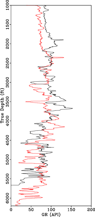
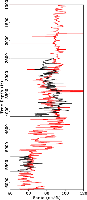
From Equation 1, to align all wells to constant geologic time, we estimate the warping function, ![]() . Because gamma ray logs are available in all wells, we use them to estimate the warping function. The deepest gamma ray log is selected as the reference log,
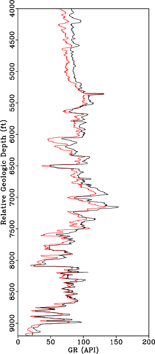
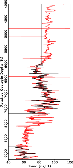
. Because gamma ray logs are available in all wells, we use them to estimate the warping function. The deepest gamma ray log is selected as the reference log, ![]() and the well containing this log is denoted by the purple star in Figure 1. The gamma ray and sonic log in the reference well are compared to the gamma ray and sonic log in a different well in Figures 8a and 8b, respectively. The shifts are estimated by matching the gamma ray log from each well to the reference gamma log as shown in Figure 9a. The alignment shifts are then applied to the remaining well logs in each well to align all well logs to constant geologic time. Results of aligning a sonic log before and after applying the shifts estimated from aligning the gamma ray logs are shown in Figures 8b and 9b, respectively.
and the well containing this log is denoted by the purple star in Figure 1. The gamma ray and sonic log in the reference well are compared to the gamma ray and sonic log in a different well in Figures 8a and 8b, respectively. The shifts are estimated by matching the gamma ray log from each well to the reference gamma log as shown in Figure 9a. The alignment shifts are then applied to the remaining well logs in each well to align all well logs to constant geologic time. Results of aligning a sonic log before and after applying the shifts estimated from aligning the gamma ray logs are shown in Figures 8b and 9b, respectively.
|
|---|
|
GR0and2,DT0and2
Figure 8. (a) Median filtered gamma log from the reference well (red) and median filtered gamma log from a second well (black) before applying alignment shifts. (b) Sonic log from the reference well (red) and sonic log from a second well (black) before applying alignment shifts. |
|
|
|
|---|
|
GR2shift0,DT2shift0
Figure 9. (a) Median filtered gamma log from the reference well (red) and an aligned gamma log from a second well (black) after applying estimated alignment shifts. (b) Sonic log from the reference well (red) and an aligned sonic log from a second well (black) after applying estimated alignment shifts from matching gamma logs. |
|
|
This approach results in well logs that are flattened along a common geologic time. The log data were collected over several years, with different logging tools, and likely different techniques applied to process the data. To account for this variability, we normalize the sonic and density logs using the big histogram method (Shier et al., 2004). For normalization, we select 15 intervals based on available well log tops and lithology variations. We estimate the cumulative mean and standard deviation for all well log data in each interval. We assume that distribution of well log data from each well, in each interval, should fall one standard deviation of the cumulative mean. With the aligned and normalized sonic logs, we estimate the missing sonic logs, or sections of sonic logs using Equation 8.
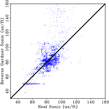
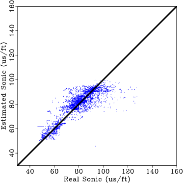
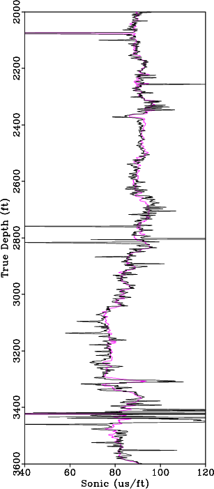
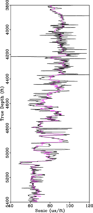
We perform a blind well test to validate the proposed approach by estimating a sonic log in a well where a real sonic log is available. For comparison, we use available density information and the Reverse Gardner Equation (Gardner et al., 1974) to estimate sonic log; this result is crossplotted against the real sonic log for the entire well in Figure 10a. When estimating the Reverse Gardner Equation, we break the well into 15 intervals based on well tops and changes in lithology from the gamma ray log, and we recompute the equation that best fits the data for each interval. The estimated sonic log using the proposed approach is crossplotted against the real sonic log for the entire well in Figure 10b. We observe significant improvement in the proposed approach over a conventional method for estimating a missing sonic log. Results comparing the sonic log estimated using the proposed approach against the real sonic log along two 1600 ft intervals are shown in Figure 11. Based on the results of our blind well test using field data, the proposed approach provides a reasonable first-order approximation of the unknown well logs and can be implemented to predict missing well log data.
|
|---|
|
xplot-DT2gard,xplot-DT2
Figure 10. (a) Real sonic log cross plotted against the sonic log estimated using Reverse Gardner equation. (b) Real sonic log cross plotted against the sonic log estimated using the proposed approach. |
|
|
|
|---|
|
DT01p0,DT02p0
Figure 11. We perform a blind well test by estimating a sonic log using the propose approach and comparing the result against the real sonic log. Real sonic log (black) versus estimated sonic log (magenta) along two 1600ft intervals along the reference log. |
|
|
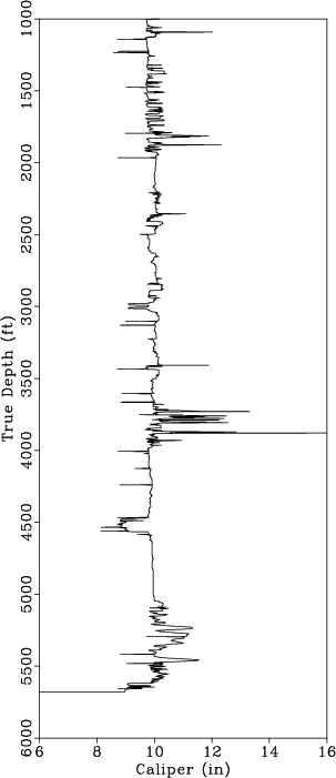
From Table 1, we observe that most wells have sonic and density log; however, the difference between the mean length of the sonic/density logs as compared to the gamma log indicates that several of the well logs were not acquired over specific intervals or have missing section as shown in Figure 9b. For well logs that have missing section or are partially complete, we include the available log data in Equation 8 to honor the available measurements and interpolate the missing log sections. In Figure 12 we interpolate missing log data where there are holes in the original log and use true well log measurements when available.


|
|---|
|
DTp2a,RHOBp2a,CAL2
Figure 12. (a) Original sonic log (black) versus estimated sonic log (magenta). (b) Original density log (black) versus estimated density log (magenta). The original well log data is used in the inversion so areas where sonic or density data is available the estimated logs match the original data. In the interval between 3500 ft and 3900 ft, there is a significant deviation in the (c) caliper log indicating an inaccurate measurement; therefore, the estimated log deviates significantly from the original log. |
|
|
We applied the proposed approach to all 26 wells from our subset of the Teapot Dome dataset to generate complete sonic and density logs for each well. Table 2 summarizes the log dataset after estimating missing or incomplete logs.
| Log Type | Wells | Sonic | Density | Caliper | Gamma |
| Number | 26 | 26 | 26 | 26 | 26 |
| Mean Length (ft) | 4192 | 3991 | 3639 | 4074 | 4074 |
By estimating missing sonic and density logs for each well, we increase the number of logs and the section of the log available to integrate with the available seismic data. Using the interpolated sonic and density logs, it is possible to compute a TDR and reflectivity series to tie any given well to seismic data.
|
|
|
|
Missing log data interpolation and semiautomatic seismic well ties using data matching techniques |