Seismic-well tie example

To demonstrate our approach, we tie 26 wells using the well log information summarized in Table 2 and the phase-adjusted 3D seismic data. Each seismic well tie is computed independently by modeling a synthetic seismogram, estimating the shifts using LSIM and computing an updated velocity function.

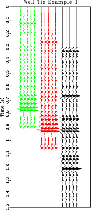
One example of a semiautomatic seismic well tie is shown in Figure 14. The synthetic modeled from the original sonic log is compared against the synthetic modeled from a sonic log updated by shifts estimated from four iterations of matching using LSIM and the closest trace from the phase adjusted seismic dataset. The high amplitude reflectors between 0.75 and 1.10 seconds are well-aligned after four iterations of shifts are estimated to update the sonic log.

synth-p3
Figure 14. Synthetic modeled using the initial sonic log (green). Synthetic modeled using the sonic log updated after four iterations of matching using LSIM to estimate shifts (red). Closest trace to the well location extracted from the phase adjusted seismic data (black).

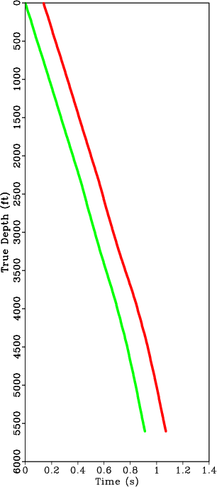
The initial Backus averaged sonic, updated sonic, and original sonic logs are shown in Figure 15a. We observe that the majority of adjustments to the sonic log occurs between 3500 and 3900 feet. This adjustment can also be observed by comparing the initial and updated TDR's in Figure 15b. The differences between synthetic seismograms modeled from well log data and seismic data are usually attributed to either inaccuracies in the seismic phase or seismic migration velocities (White, 1998; Henry, 2000). The bulk shift between initial and final TDR is related to missing shallow velocity section in the well log. The results in Figure 15 provide an initial qualitative assessment of a seismic well tie to ensure the estimated shifts do not result in an improbable update to the sonic log. We overlay the modeled and tied synthetic seismogram with the crossline that cuts through the well and observe a reasonable tie with the seismic data, even in the presence of a fault (Figure 16).

DTpi3,tdr3
Figure 15. (a) Estimated sonic log using the proposed approach after Backus averaging (green). Updated sonic log after four iterations of matching using LSIM to estimate shifts (red). Estimated sonic log after interpolation of missing data (black). (b) TDR from estimated sonic log (green). Updated TDR after four iterations of matching using LSIM to estimate shifts (red).

inline3
Figure 16. Seismic crossline through well in Figures 14 and 15. We observe a good tie between the modeled synthetic and real seismic data. The sonic and density logs used to model the synthetic are estimated using the proposed approach.