next up previous [pdf]

Next: Nankai field data example Up: Examples Previous: Examples

Linear-gradient model

We start with a toy example of a linear-gradient model similar to the one used by Baina et al. (2002). The velocity in Figure 1a changes with a constant gradient tilted at $45^{\circ}$. In this model, the exact velocity is given by
\begin{displaymath}
v (x,z) = v_0 + g_z z + g_x x\;,
\end{displaymath} (22)

where $v_0 = 1$ km/s, $g_z = 0.15$ 1/s, and $g_x=0.15$ 1/s. Four reflectors with varying shapes are embedded in the model. Reflection data in Figure 1b are modeled using the Kirchhoff modeling. The migration velocity squared $w_m$ and its Dix-inverted counterpart $w_d$ are given by the following expression (Li and Fomel, 2015)
$\displaystyle w_m (x_0,t_0)$ $\textstyle =$ $\displaystyle \left(\frac{(v_0 + g_x x_0)^2}{t_0 \left( g \coth (g t_0) - g_z \right)} \right)^2~,$ (23)
$\displaystyle w_d (x_0,t_0)$ $\textstyle =$ $\displaystyle \left(\frac{(v_0 + g_x x_0) g}{g \cosh (g t_0) - g_z \sinh (g t_0)}\right)^2~.$ (24)

The time-migration velocity computed using the analytical expression from Li and Fomel (2015) is shown in Figure 2a. The Kirchhoff time migration in Figure 2b fails to focus the image accurately because of strong lateral velocity variations. Figure 3a shows the Dix velocity that we further use to obtain the image by wave-equation time migration using reverse-time migration in image-ray coordinates (Dell et al., 2014) as shown in Figure 3b. The image is correctly focused but distorted because of image-ray bending. Bending image rays in Figure 4a correspond to the time-migration velocity shown in Figure 2a. The analytical solutions to time-to-depth conversion are (Li and Fomel, 2015)
$\displaystyle x_0 (x,z)$ $\textstyle =$ $\displaystyle x + \frac{\sqrt{(v_0+g_x x)^2 + g_x^2 z^2} - (v_0 + g_x x)}{g_x}~,$ (25)
$\displaystyle t_0 (x,z)$ $\textstyle =$ $\displaystyle \frac{1}{g} \mathrm{arccosh} \left[ \frac{g^2 \left( \sqrt{(v_0+g_x x)^2 + g_x^2 z^2} + g_z z \right) - v g_z^2}{v g_x^2} \right]~.$ (26)

Figure 4b shows time-migration images converted to Cartesian coordinates. The image by wave-equation time migration is now both well focused, correctly positioned in depth, and is comparable in quality to the depth migrated image in Figure 4c. Both images are created using low-rank reverse-time migration (Fomel et al., 2013).

vel zodata
vel,zodata
Figure 1.
Simple synthetic model (a) Velocity model. (b) Zero-offset data.
[pdf] [pdf] [png] [png] [scons]

vmigwin kpstmtime
vmigwin,kpstmtime
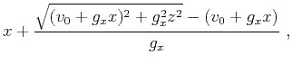
Figure 2.
(a) Time migration velocity, and (b) Image obtained by Kirchhoff time migration.
[pdf] [pdf] [png] [png] [scons]

vdix wetm1
vdix,wetm1
Figure 3.
(a) Dix velocity, and (b) Image obtained by wave-equation time migration using RTM in image-ray coordinates. All events are correctly focused in image-ray coordinates but appear in a distorted coordinate frame.
[pdf] [pdf] [png] [png] [scons]

acoord anamapd zomig
acoord,anamapd,zomig
Figure 4.
(a) Image rays (curves of constant $x_0$) and wavefronts (curves of constant $t_0$). (b) Image obtained using wave-equation time migration after conversion to Cartesian coordinates, and (c) Image obtained using depth migration using RTM in Cartesian coordinates.
[pdf] [pdf] [pdf] [png] [png] [png] [scons]


next up previous [pdf]

Next: Nankai field data example Up: Examples Previous: Examples

2022-05-23