 |
 |
 |
 | Simulating propagation of separated wave modes in general anisotropic media,
Part II: qS-wave propagators |  |
![[pdf]](icons/pdf.png) |
Next: Pure-mode SH-wave equation
Up: Cheng & Kang: Propagate
Previous: Introduction
Following Carcione (2007),
we denote the spatial variables  ,
,  and
and  of a Cartesian system by
the indices
of a Cartesian system by
the indices  ...
... ,
,  and
and  , respectively, the position vector by
 , a partial derivative with respect to a variable
  with
with
 ,
and the first and second time derivatives with
,
and the first and second time derivatives with
 and
and
 .
Matrix transposition is denoted by the superscript
.
Matrix transposition is denoted by the superscript  . We also denote
the scalar and matrix products by the symbol
. We also denote
the scalar and matrix products by the symbol  , and the gradient operator by
 .
.
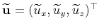
The wave equation in a general heterogeneous anisotropic medium can be expressed as
![$\displaystyle \rho{\partial_{tt}\mathbf{u}} = [{\bigtriangledown}{\mathbf{C}{\bigtriangledown}^{\top}}]\mathbf{u} + \mathbf{f},$](img28.png) |
(1) |
where
 is the particle displacement vector,
 represents
the force term,
represents
the force term,  the density,
 the matrix representing the stiffness tensor in a
two-index notation called the “Voigt recipe”. The gradient operator has
the following matrix representation:
the matrix representing the stiffness tensor in a
two-index notation called the “Voigt recipe”. The gradient operator has
the following matrix representation:
 |
(2) |
Neglecting the source term, a plane-wave analysis of the elastic wave equation yields the
Christoffel equation,
 |
(3) |
where  is the angular frequency and
 is the wavefield in Fourier domain; the wavenumber-domain counterpart of the gradient
operator is written as
is the wavefield in Fourier domain; the wavenumber-domain counterpart of the gradient
operator is written as
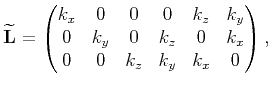 |
(4) |
in which the propagation direction is specified by the wave vector
 ,
and the symmetric Christoffel matrix
,
and the symmetric Christoffel matrix
 satisfies:
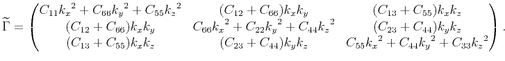 |
(5) |
The squared phase (or normal) velocities
 are eigenvalues of the
Christoffel matrix. The inequalitities
are eigenvalues of the
Christoffel matrix. The inequalitities
 |
(6) |
establish the types of waves.
Except for anomalous cases of elastic anisotropy, which are of little interest in geophysics,
the qP-wave ( ) usually is faster than qS-waves (
 )
and the equation
)
and the equation
 |
(7) |
is a great rarity (Yu et al., 1993). However, the equation
 |
(8) |
is a common event because the phase velocity surfaces (corresponding to qS1 and qS2 waves) can touch or intersect each other (Musgrave, 1970).
Directions of wave normals along which the two phase velocities are equal to each other are called acoustic axes or singularity directions.
For the shear singularities, the Christoffel matrix is degenerate.
Crampin (1991) distinguished three kinds of singularity: point, kiss and line.
In point and kiss singularities, the phase velocity surfaces touch at a single point, while in line singularities
they intersect.
Generally, inserting a nondegenerate eigenvalue back into the Christoffel equation gives ratios of
the components of
 ,
which specify polarization along a given phase direction for a given wave mode.
The polarization consists of the geometrical properties of the particle motion, including trajectory shape and spatial orientation,
but excludes magnitudes of the motion.
Polarization of an isolated body wave in a noise-free perfectly elastic medium is linear (Winterstein, 1990).
In isotropic media, polarizations of such body waves are either parallel to the direction of wave travel, for P-waves,
or perpendicular to it, for S-waves. The polarization vectors of the S-wave may take an arbitrary orientation in the
plane orthogonal to the P-wave polarization vector.
In anisotropic media, however, the polarizations are often neither parallel nor
perpendicular to the direction of wave propagation.
Whether the medium is anisotropic or not, the polarizations of the three wave modes are always mutually orthogonal for a given propagation direction.
So we may separate the elastic wavefield into single-mode scalar fields using the polarization-based projection:
,
which specify polarization along a given phase direction for a given wave mode.
The polarization consists of the geometrical properties of the particle motion, including trajectory shape and spatial orientation,
but excludes magnitudes of the motion.
Polarization of an isolated body wave in a noise-free perfectly elastic medium is linear (Winterstein, 1990).
In isotropic media, polarizations of such body waves are either parallel to the direction of wave travel, for P-waves,
or perpendicular to it, for S-waves. The polarization vectors of the S-wave may take an arbitrary orientation in the
plane orthogonal to the P-wave polarization vector.
In anisotropic media, however, the polarizations are often neither parallel nor
perpendicular to the direction of wave propagation.
Whether the medium is anisotropic or not, the polarizations of the three wave modes are always mutually orthogonal for a given propagation direction.
So we may separate the elastic wavefield into single-mode scalar fields using the polarization-based projection:
 |
(9) |
with
 representing the normalized polarization vector of the given mode
 (Dellinger, 1991).
In practice, horizontally polarized (or SH) and vertically polarized (or SV) are
likely to be the most useful S-wave modes when consideration is restricted to isotropic or TI media,
in which all rays lie in symmetry planes.
For isotropic media, the above polarization-based projection is material-independent,
because the following vectors related to the wave vector
 , i.e.,
 and and |
(10) |
indicate the polarization direction of pure P-, SH- and SV-wave, respectively.
On the contrary, for anisotropic media, the polarization-based projection depends on local material parameters,
because the polarizations are generally specified by the eigenvectors of the original Christoffel equation.
For a VTI medium, the stiffness coefficients satisfy:
 ,
,
 ,
,
 and
and
 .
In this case, people still prefer to designate the qS-waves as SH-like and SV-like modes due to the following fact:
The use of qS1 and qS2 distinguished by phase velocities does not always give continuous polarization surfaces,
while the use of SV and SH distinguished by polarization does, except at the kiss singularity at
.
In this case, people still prefer to designate the qS-waves as SH-like and SV-like modes due to the following fact:
The use of qS1 and qS2 distinguished by phase velocities does not always give continuous polarization surfaces,
while the use of SV and SH distinguished by polarization does, except at the kiss singularity at 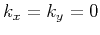 (Crampin and Yedlin, 1981; Zhang and McMechan, 2010).
In this case, the SH-waves polarize perpendicular to the symmetry plane and are pure,
and the SV-waves polarize in symmetry planes and are usually quasi-shear.
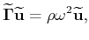
As shown in Figure 1, for both qP and qSV modes, the polarization directions in a VTI material
deviate from those in the corresponding isotropic (reference) medium in most propagation directions,
but no deviation exists for the SH mode in any direction for either medium.
To our interest, the polarization deviations of qP- or qSV-waves between an ordinary VTI
medium and its isotropic reference are usually very small, although exceptions are possible (Tsvankin and Chesnokov, 1990; Thomsen, 1986).
In addition, taking vectors
(Crampin and Yedlin, 1981; Zhang and McMechan, 2010).
In this case, the SH-waves polarize perpendicular to the symmetry plane and are pure,
and the SV-waves polarize in symmetry planes and are usually quasi-shear.
As shown in Figure 1, for both qP and qSV modes, the polarization directions in a VTI material
deviate from those in the corresponding isotropic (reference) medium in most propagation directions,
but no deviation exists for the SH mode in any direction for either medium.
To our interest, the polarization deviations of qP- or qSV-waves between an ordinary VTI
medium and its isotropic reference are usually very small, although exceptions are possible (Tsvankin and Chesnokov, 1990; Thomsen, 1986).
In addition, taking vectors
 ,
,
 and
and
 as the three mutually perpendicular polarization vectors
in the unperturbed isotropic medium, approximate formulas for the qP- and qS-wave polarizations
in an arbitrary anisotropic medium can be developed using perturbation theory (Cerveny and Jech, 1982; Farra, 2001; Psencik and Gajewski, 1998).
as the three mutually perpendicular polarization vectors
in the unperturbed isotropic medium, approximate formulas for the qP- and qS-wave polarizations
in an arbitrary anisotropic medium can be developed using perturbation theory (Cerveny and Jech, 1982; Farra, 2001; Psencik and Gajewski, 1998).


|
|---|
P_last,SV_last,SH_last
Figure 1.
Polarization vectors in a 3D VTI material with
 km/s,
km/s,
 km/s,
km/s,
 , and
, and
 . Its isotropic reference
medium is determined by setting
. Its isotropic reference
medium is determined by setting
 and
and  .
One can observe polarization deviations between VTI (red) and its isotropic reference (blue) media for (a) P- and (b) S-waves in
most propagation directions, but no deviation for (c) SH-waves in any direction.
.
One can observe polarization deviations between VTI (red) and its isotropic reference (blue) media for (a) P- and (b) S-waves in
most propagation directions, but no deviation for (c) SH-waves in any direction.
|
|---|
![[png]](icons/viewmag.png)
|
|---|
To provide for more possibilities and flexibility in describing single-mode wave propagation in anisotropic media, Cheng and Kang (2014) suggest splitting
the one-step polarization-based projection into two steps, of which the first step implicitly implements partial wave-mode separation
during wavefield extrapolation with a transformed wave equation, while the second step is designed to correct the
projection deviation due to the approximation of polarization directions.
The transformed wave equation (that they called a pseudo-pure-mode qP-wave equation) was derived from the original Christoffel equation through
a similarity transformation aiming to project the displacement wavefield onto the isotropic (reference) polarization direction indicated by
.
In this paper, taking another two orthogonal vectors in equation 10, namely
and
,
as the reference polarization directions for SH- and qSV-waves,
we apply the same strategy to derive simplified wave equations for these qS-wave modes in general TI media.
|
|
|
|
| Simulating propagation of separated wave modes in general anisotropic media,
Part II: qS-wave propagators | |
|
Next: Pure-mode SH-wave equation
Up: Cheng & Kang: Propagate
Previous: Introduction
2016-10-14