|
|
|
|
A graphics processing unit implementation of time-domain full-waveform inversion |
One key problem of GPU-based implementations of FWI is that the computation is always much faster than the data transfer between the host and device. Many researchers choose to reconstruct the source wavefield instead of storing the modeling time history on the disk, just saving the boundaries (Dussaud et al., 2008; Yang et al., 2014). For ![]() -th order finite difference, regular grid scheme needs to save
-th order finite difference, regular grid scheme needs to save ![]() points on each side (Dussaud et al., 2008), while staggered-grid scheme required at least
points on each side (Dussaud et al., 2008), while staggered-grid scheme required at least ![]() points on each side (Yang et al., 2014). In our implementation, we use 2nd order regular grid finite difference because FWI begins with a rough model and velocity refinement is mainly carried out during the optimization. Furthermore, high-order finite differences and staggered-grid schemes do not necessarily lead to FWI converge to an accurate solution while requiring more compute resources. A key observation for wavefield reconstruction is that one can reuse the same template by exchanging the role of
points on each side (Yang et al., 2014). In our implementation, we use 2nd order regular grid finite difference because FWI begins with a rough model and velocity refinement is mainly carried out during the optimization. Furthermore, high-order finite differences and staggered-grid schemes do not necessarily lead to FWI converge to an accurate solution while requiring more compute resources. A key observation for wavefield reconstruction is that one can reuse the same template by exchanging the role of ![]() and
and ![]() . In other words, for forward modeling we use
. In other words, for forward modeling we use
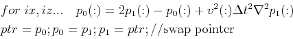 |
(15) |
Note that all the computation is done on GPU blocks. In our codes, the size of the block is set to be 16x16. We replicate the right- and bottom-most cols/rows enough times to bring the total model size up to an even multiple of block size. As shown in Figure 2, the whole computation area is divided into 16x16 blocks. For each block, we use a 18x18 shared memory array to cover all the grid points in this block. It implies that we add a redundant point on each side, which stores the value from other blocks, as marked by the window in Figure 2. When the computation is not performed for the interior blocks, special care needs to be paid to the choice of absorbing boundary condition (ABC) in the design of FWI codes. Allowing for efficient GPU implementation, we use the ![]() Clayton-Enquist ABC proposed in Clayton and Engquist (1977) and Engquist and Majda (1977). For the left boundary, it is
Clayton-Enquist ABC proposed in Clayton and Engquist (1977) and Engquist and Majda (1977). For the left boundary, it is
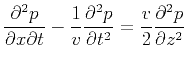 |
(16) |

|
|---|
|
blocks
Figure 2. 2D blocks in GPU memory. The marked window indicates that the shared memory in every block needs to be extended on each side with halo ghost points storing the grid value from other blocks. |
|
|
|
|
|
|
A graphics processing unit implementation of time-domain full-waveform inversion |