Examples

We first apply the proposed optimal rank-reduction method to a 5D synthetic data with linear/planar events, as shown in Figure 1. Figure 1(a) shows the clean synthetic data in a common offset gather. The 3D common offset gather ($t-x-y$) has been arranged into a 2D matrix. Figure 1(b) shows the noisy data with extremely strong band-limited random noise. The useful signals are almost buried in the strong noise. Figure 1(c) shows the incomplete data, where 75% traces have been randomly decimated. The reconstructed and denoised data using three different methods, i.e., the traditional rank-reduction method (RR), the damped rank-reduction method (DRR), and the optimally damped rank-reduction method (ORR), are shown in Figure 2. All three methods successfully recovered most of the signals. It is clear that the RR method causes significant residual noise, the result from the DRR method is much cleaner than that from the RR method but still contains some residual noise. The proposed ORR method, however, obtains the cleanest result among the three results shown in Figure 2. To evaluate the quality of the three reconstructed data, given the exact solution in Figure 1(a), we calculate the local similarity map between each reconstructed data and the exact solution. The local similarity is a way to evaluate the similarity between two vectors/matrices/cubes in a local manner so that the evaluation can be revealed immediately from the calculated local similarity maps. The detailed introduction of mathematics behind the local similarity calculation can be found in Chen and Fomel (2015). From the local similarity comparison, it is quite obvious that from the top panel (RR method) to the bottom panel (ORR method), the similarity becomes higher and higher, which indicates that the proposed method obtains the most accurate solution.

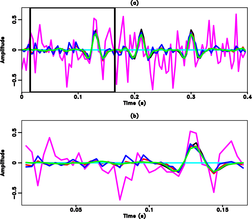
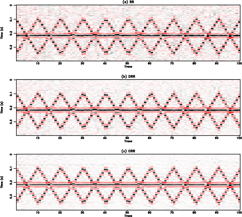
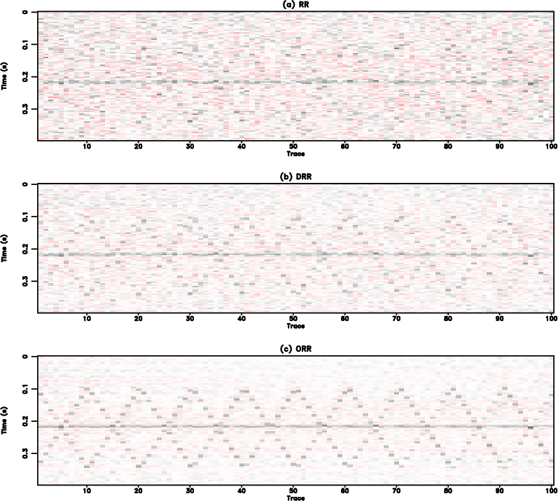
To examine the amplitude recovery quality, we select the 22nd traces from the clean data in Figure 1(a) and from the three reconstructed data in Figure 2, and draw them in Figure 4. Figure 4(a) shows the trace-by-trace comparison in the range of the whole trace and Figure 4(b) shows the zoomed trade-by-trace comparison. The zooming part is highlighted by the red transparent rectangle shown in Figure 4(a). From Figure 4 we can see that both RR and DRR methods (blue and red lines) cause strong fluctuations in the front part of the trace, while the proposed method obtains a result (the green line) that is the closest to the exact solution (the black line). The observation is even clearer in the zoomed comparison shown in Figure 4(b). Figure 5 shows the comparison of reconstruction error. The reconstruction error is calculated as the difference between the exact solution (Figure 1(a)) and each reconstructed data shown in Figure 2. From Figure 5 we can observe that both RR and DRR cause significant error and the proposed ORR method causes negligible reconstruction error except for some observable signal energy. The reconstruction error of RR method is higher than the DRR method, mostly because of the stronger residual noise caused by the RR method. Since the reconstruction error for the proposed method is mostly negligible, the error caused by the leakage signal energy becomes more apparent. To compare the leakage signal energy among three methods, we calculate the extra noise section of the RR and DRR methods. The extra noise section refers to the extra noise compared with the reference noise section from the ORR method (Figure 5(c)), thus is calculated as the difference between the error from either RR or DRR method and the error from the ORR method. The extra noise sections corresponding to the RR and DRR methods are shown in Figure 6. It is obvious that by calculating the extra error sections, the leakage useful energy from RR/DRR method and ORR method counteract each other and the resulting sections are mostly random noise. This observation indicates that the energy of the leakage signal for the three methods are nearly the same. We conclude from this test that despite the same damage to useful signals, the proposed method causes the least residual noise and thus obtains the cleanest reconstruction result.

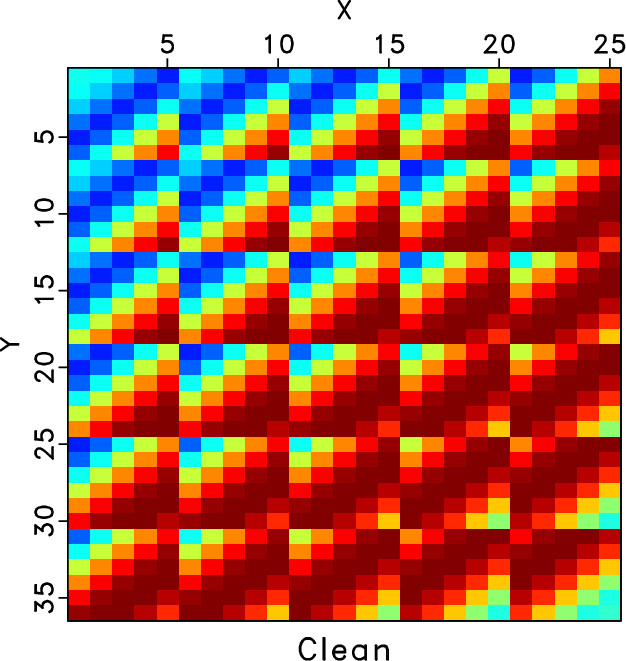
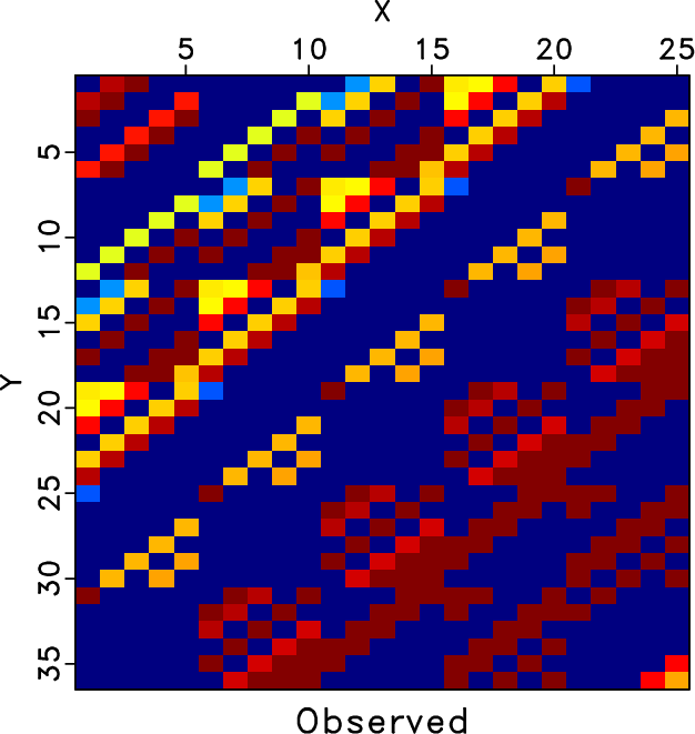
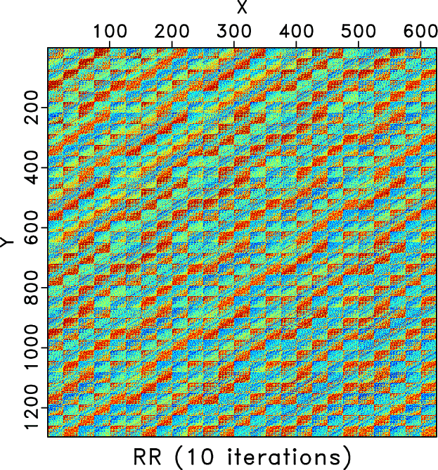
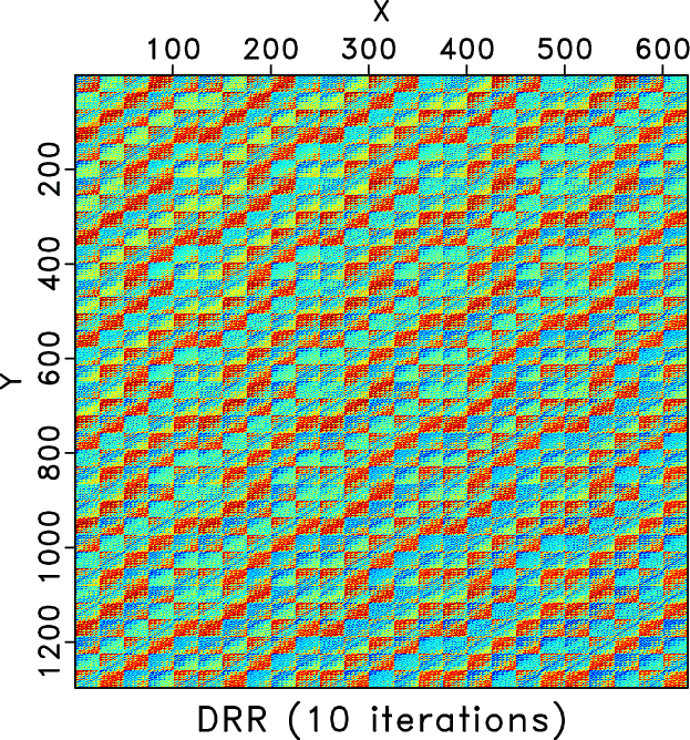
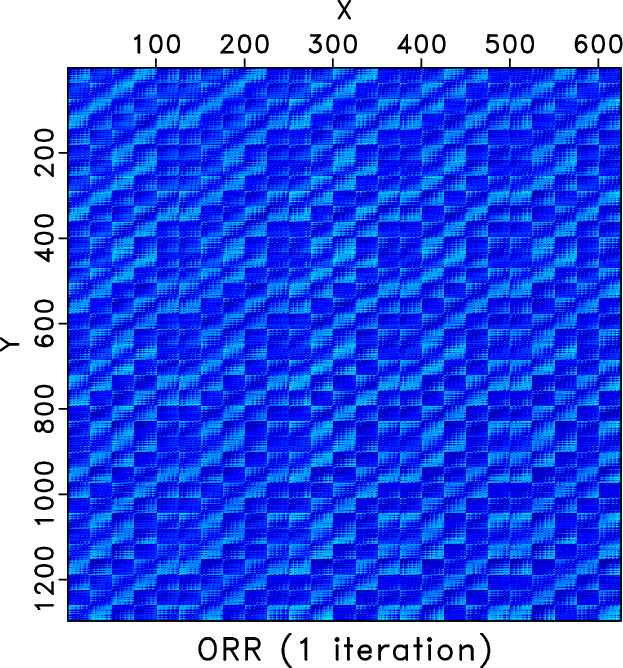
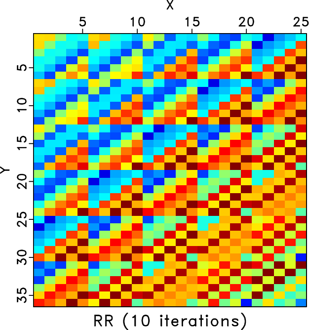
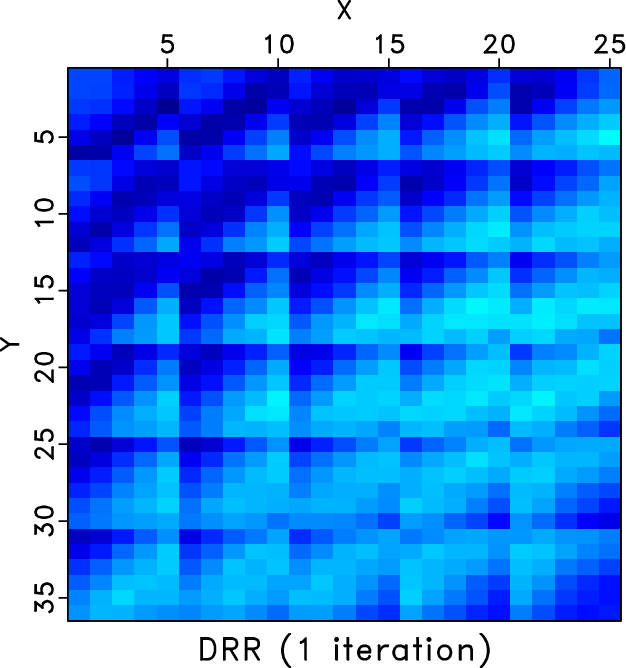
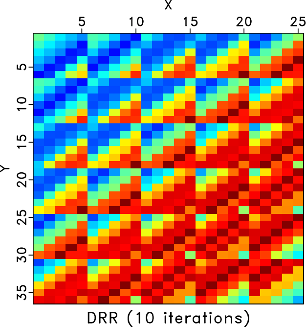
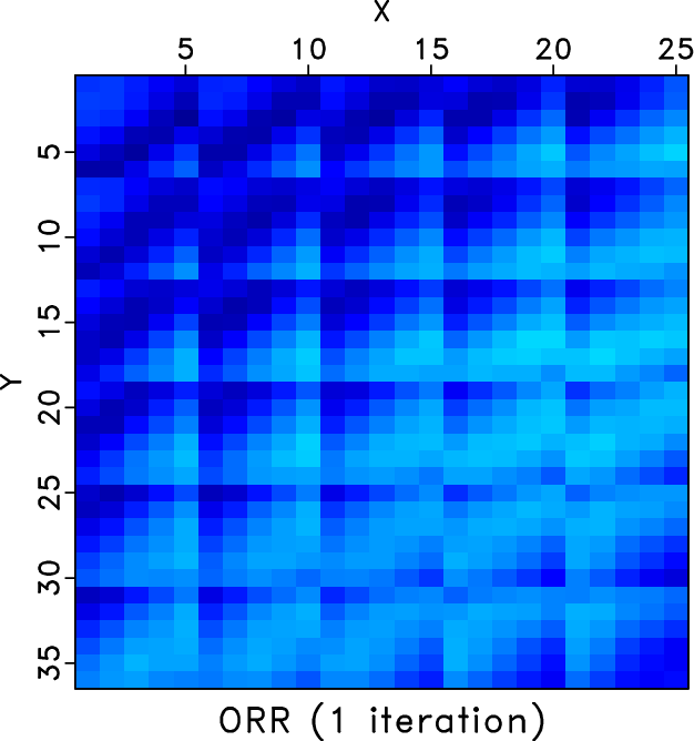
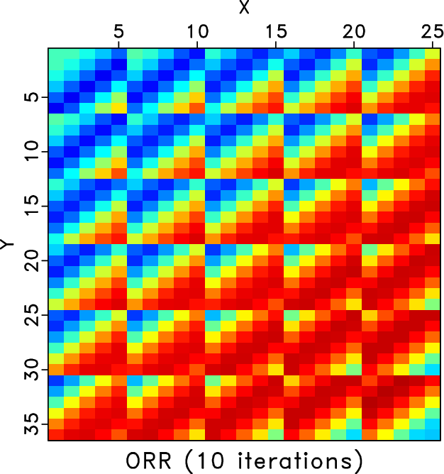
We also compare the level-four block Hankel matrices of different methods. Figures 7a and 7b shows the Hankel matrices for the clean and incomplete data for the frequency slice of 30Hz. Figures 7c and 7d show the zoomed Hankel matrices for the clean and incomplete data. The zooming areas are highlighted by the red rectangles shown in Figures 7a and 7b. Because of the missing traces, the Hankel matrix contains a number of blank areas. Figure 8 shows the Hankel matrices for different methods. The left column correspond to the Hankel matrices after 1 iteration. The right column correspond to the Hankel matrices after 10 iterations. We only conclude from Figure 8 that after 10 iterations all three methods obtain similar Hankel matrices as the exact solution shown in Figure 7a but we cannot see the difference between different methods clearly. The differences between different methods can be clearly observed from the zoomed Hankel matrices, as shown in Figure 9. It is clear that from the top to bottom in Figure 9, the Hankel matrix becomes smoother and smoother and is closer to the exact solution shown in Figure 7c.

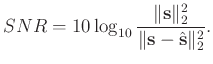
In addition to the local similarity mentioned above, we also use the signal-to-noise ratio (SNR) defined as follows to quantitatively measure the performance (Chen, 2017; Huang et al., 2017,2016):

$$SNR=10\log_{10}\frac{\Arrowvert \mathbf{s} \Arrowvert_2^2}{\Arrowvert \mathbf{s} -\hat{\mathbf{s}}\Arrowvert_2^2}.$$ (34)

where $\mathbf{s}$ denotes the vectorized clean data and $\hat{\mathbf{s}}$ denotes the vectorized reconstructed data. In this example, the SNRs of the observed data, the reconstructed results via the RR method, the DRR method, and ORR method are -4.59 dB, 5.51 dB, 9.54 dB, and 11.83 dB, respectively. In this test, we use $rank=10$, assuming that we do not have a prior information about the structural complexity of the data and thus needing to set a relatively high rank. We then test the performance when the rank is chosen smaller. The reconstructed data when $rank=5$ are shown in Figure 10. Their corresponding error sections are shown in Figure 11. From Figures 10 and 11, we can reach almost the same conclusion as the last test. In this case, the SNRs of the reconstructed results via the RR method, the DRR method, and ORR method are 8.01 dB, 10.87 dB, and 11.97 dB, respectively. The detailed SNR comparison is shown in Table 1, including the case when $rank=3$.

figure1
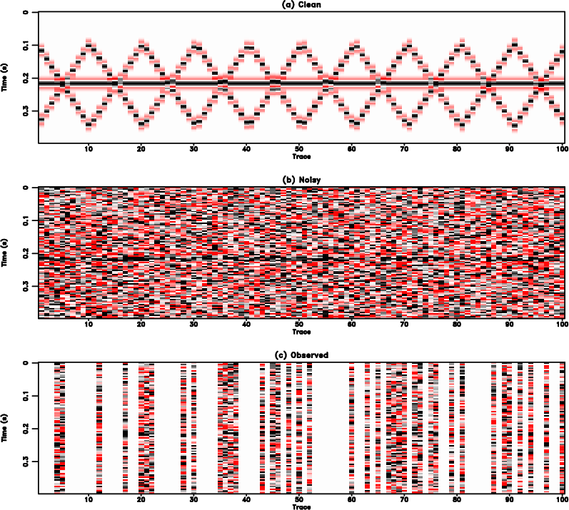
Figure 1. Common offset gather comparison for the synthetic example (reshaped into a 2-D matrix). (a) Clean data. (b) Noisy data. Note that because of the strong random noise, the useful signals are almost buried in the noise. (c) Incomplete data with 70% randomly removed traces. The blanks in (c) indicate where there are missing traces. The strong noise and missing traces make the data quality extremely low.

figure2
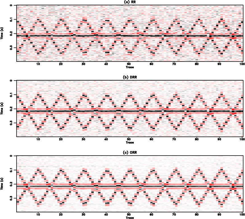
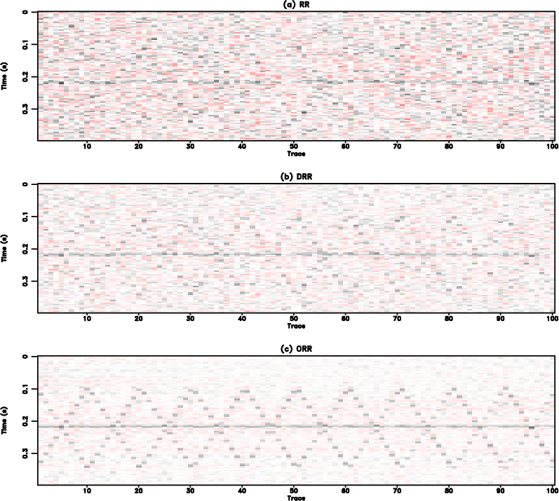
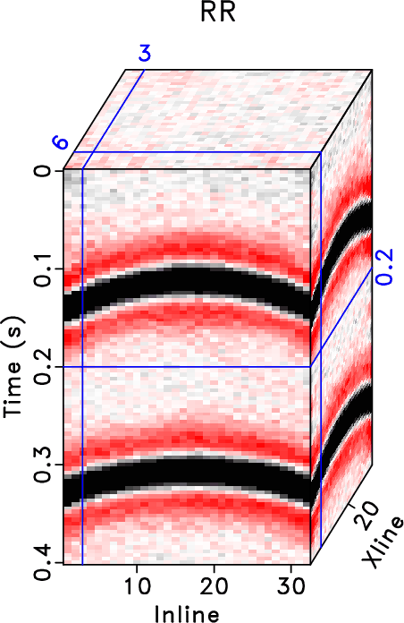
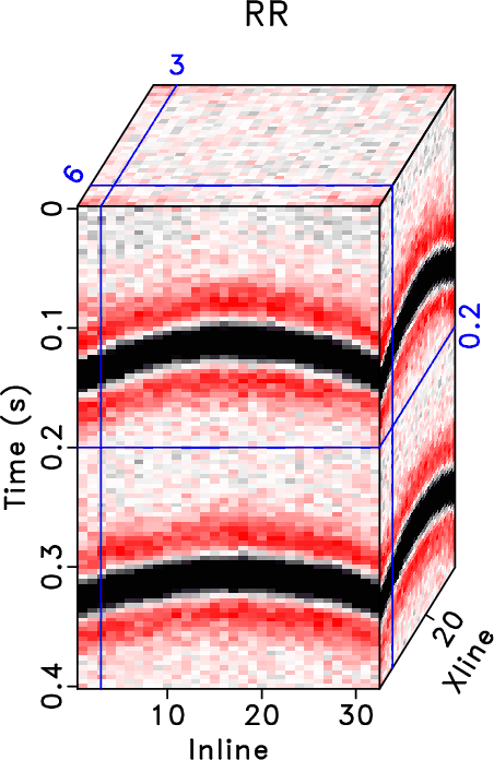
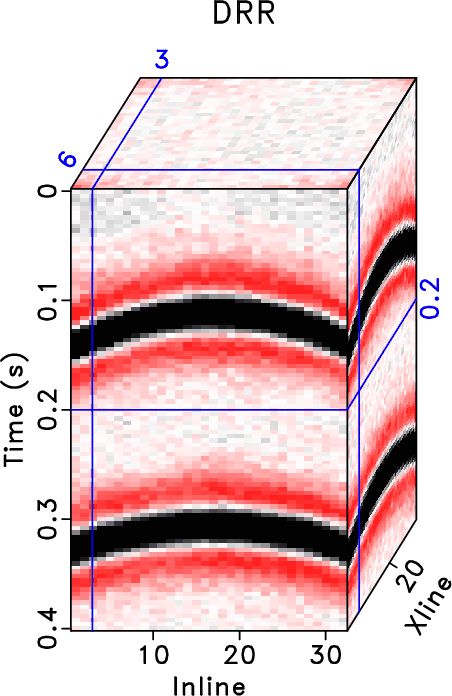
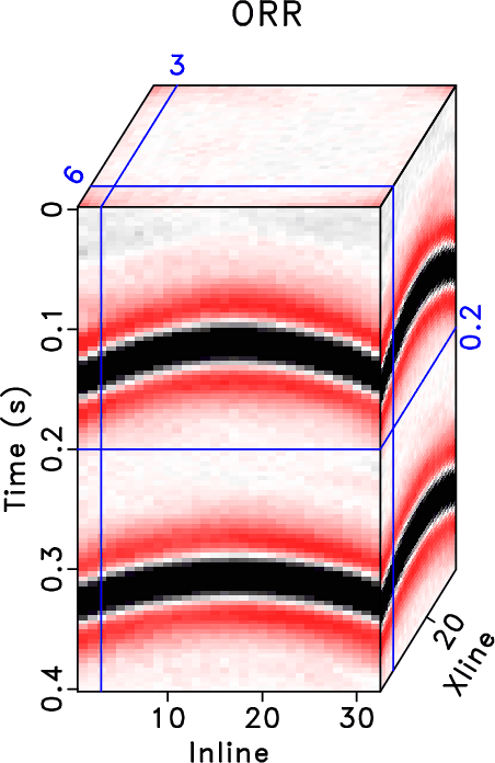
Figure 2. Common offset gather comparison for the synthetic example (reshaped into a 2-D matrix). (a) Reconstructed data using the RR method. (b) Reconstructed data using the DRR method. (c) Reconstructed data using the ORR method. In this case, $rank=10$.

figure3
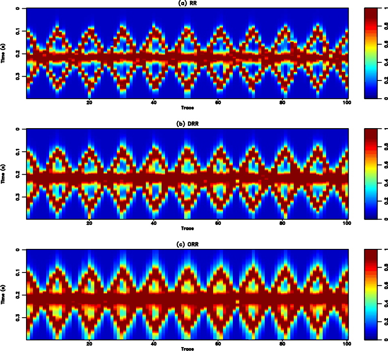
Figure 3. Local similarity comparison for the synthetic example (reshaped into a 2-D matrix). (a) Local similarity using the RR method. (b) Local similarity using the DRR method. (c) Local similarity using the ORR method. It is obvious that the local similarity of the ORR method is much larger than the other two methods, indicating a more accurate reconstruction performance.

figure4
Figure 4. Trace-by-trace comparison. (a) Comparison in the whole trace. The black line denotes the exact solution. Green line denotes the result from the proposed method. Red line denotes the result from the DRR method. Blue line denotes the result from the RR method. (b) Zoomed trace from (a). The transparant red window highlight the zooming area.

figure5
Figure 5. Common offset gather comparison for the synthetic example (reshaped into a 2-D matrix). (a) Reconstruction error using the RR method. (b) Reconstruction error using the DRR method. (c) Reconstruction error using the ORR method. In this case, $rank=10$.

figure6
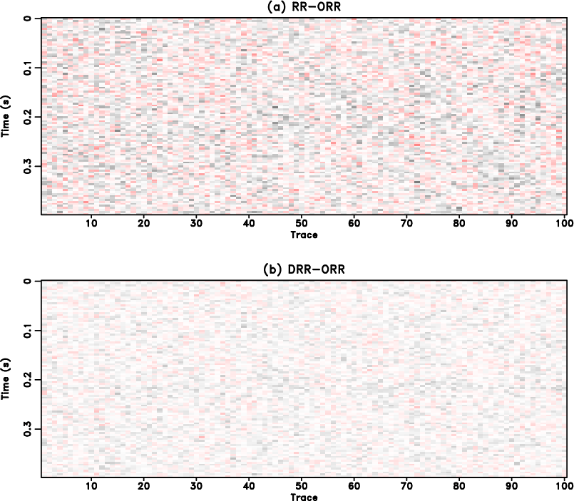
Figure 6. Extra error comparison compared with the ORR method for the synthetic example (reshaped into a 2-D matrix) when $rank=10$. (a) Extra error caused by RR method (the difference between 5(a) and 5(c)). (b) Extra error caused by RR method (the difference between 5(b) and 5(c)).

H_clean,H_obs,H-z-clean,H-z-obs
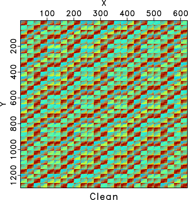
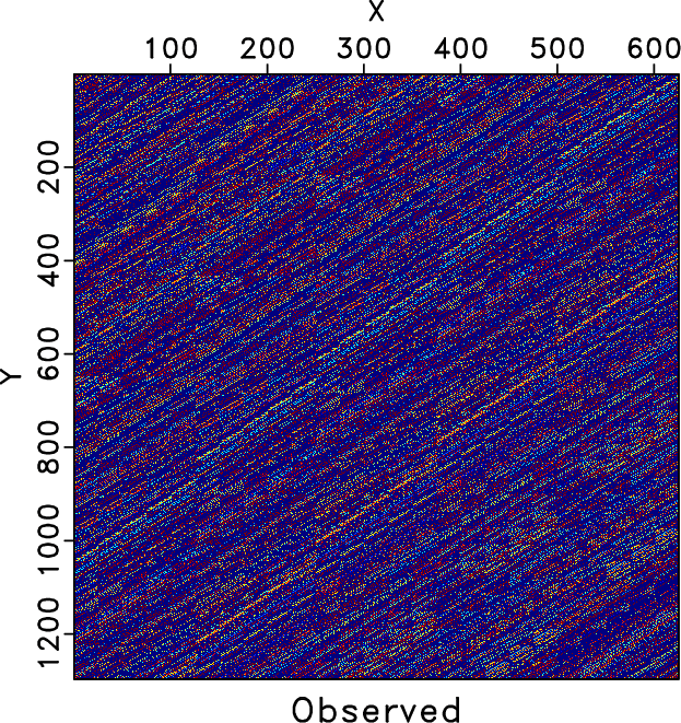
Figure 7. Hankel matrices for the clean and observed data for frequency slice of 30Hz. (a) Hankel matrix of the clean data. (b) Hankel matrix of the observed data. (c) & (d) Zoomed Hankel matrices of (a) & (b). The zooming area is highlighted by the red rectangles.

H_rr1,H_rr10,H_drr1,H_drr10,H_odrr1,H_odrr10
Figure 8. Hankel matrices for different methods for frequency slice of 30Hz. Left column: Hankel matrix after 1 iteration. Right: Hankel matrix after 10 iterations. Top row: Hankel matrices for the RR method. Middle row: Hankel matrix for the DRR method. Bottom row: Hankel matrix for the ORR method.

H-z-rr1,H-z-rr10,H-z-drr1,H-z-drr10,H-z-odrr1,H-z-odrr10
Figure 9. Zoomed Hankel matrices for different methods for frequency slice of 30Hz. Left column: Hankel matrix after 1 iteration. Right: Hankel matrix after 10 iterations. Top row: Hankel matrices for the RR method. Middle row: Hankel matrix for the DRR method. Bottom row: Hankel matrix for the ORR method.

figure10
Figure 10. Common offset gather comparison for the synthetic example (reshaped into a 2-D matrix). (a) Reconstructed data using the RR method. (b) Reconstructed data using the DRR method. (c) Reconstructed data using the ORR method. In this case, $rank=5$.

figure11
Figure 11. Common offset gather comparison for the synthetic example (reshaped into a 2-D matrix). (a) Reconstruction error using the RR method. (b) Reconstruction error using the DRR method. (c) Reconstruction error using the ORR method. In this case, $rank=5$.

snr-n
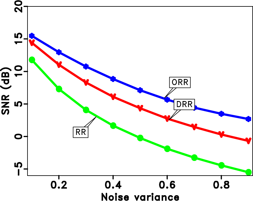
Figure 12. SNR diagrams of the different approaches with respect to the noise level (variance value). Note that the proposed approach outperforms the traditional methods more and more as the noise level increases.

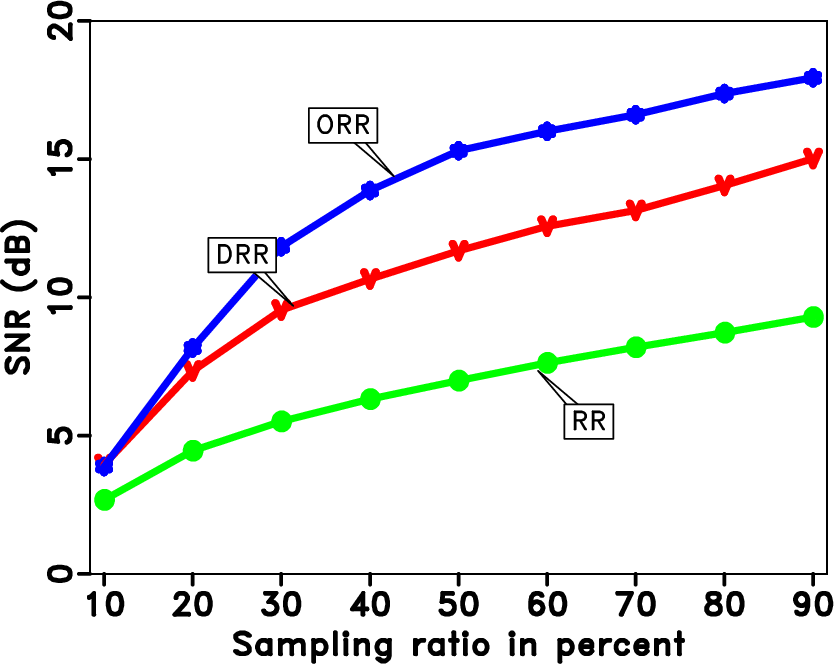
snr-r
Figure 13. SNR diagrams of the different approaches with respect to the sampling ratio (in percent). It is obvious that the difference between the ORR method and the DRR method becomes larger as the sampling ratio increases. The ORR method always outperforms the other methods for all sampling ratios.

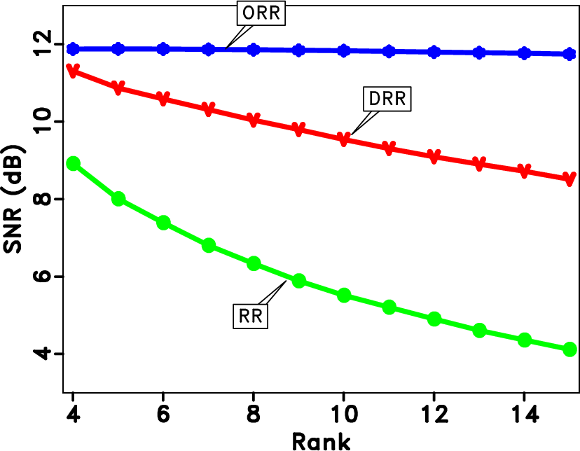
snr-rank
Figure 14. SNR diagrams of the different approaches with respect to the selected rank. The ORR method is obviously much less sensitive to the rank compared with other two methods. This phenomenon indicates that the ORR method can be applied as an adaptive method by setting a relatively large rank.

hyper-clean-hxhy,hyper-noisy-hxhy,hyper-obs-hxhy
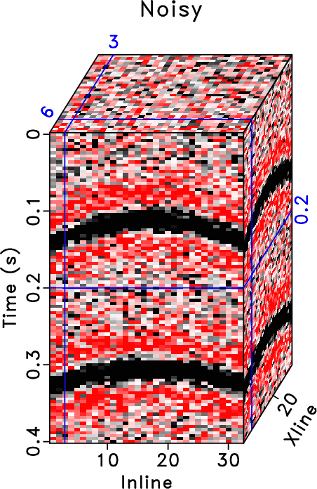
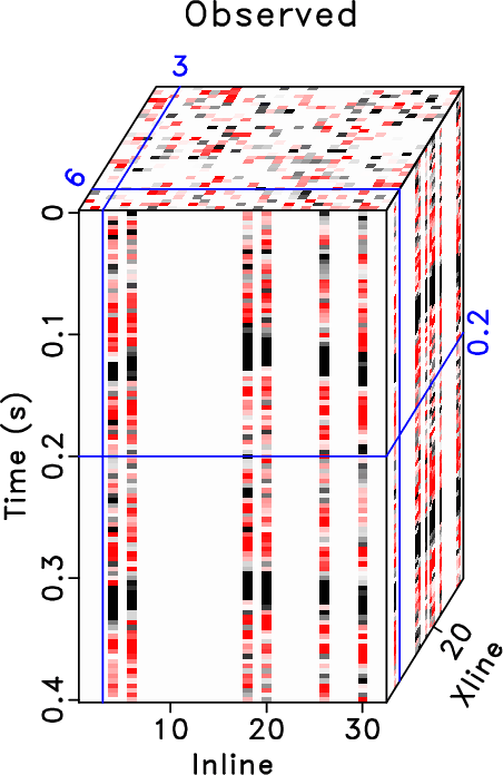
Figure 15. Common midpoint gather comparison for the synthetic example with hyperbolic events. (a) Clean data. (b) Noisy data. (c) Incomplete data. The blanks in (c) indicate where there are missing traces.

hyper-rr-hxhy,hyper-drr-hxhy,hyper-odrr-hxhy,hyper-rr2-hxhy,hyper-drr2-hxhy,hyper-odrr2-hxhy
Figure 16. Common midpoint gather comparison for the synthetic example with hyperbolic events. Top row shows results when $rank=12$. Bottom row shows results when $rank=24$. Left: Reconstructed data using the RR method. Middle: Reconstructed data using the DRR method. Right Reconstructed data using the ORR method. The SNR comparisons are shown in Table 3.

hyper-rr-hxhy-simi,hyper-drr-hxhy-simi,hyper-odrr-hxhy-simi,hyper-rr2-hxhy-simi,hyper-drr2-hxhy-simi,hyper-odrr2-hxhy-simi
Figure 17. Local similarity comparison for the synthetic example with hyperbolic events. Top row shows results when $rank=12$. Bottom row shows results when $rank=24$. Left: Reconstructed data using the RR method. Middle: Reconstructed data using the DRR method. Right Reconstructed data using the ORR method. The introduction of local similarity is given in Chen and Fomel (2015).

field_d0_0
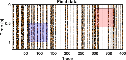
Figure 18. Real data example with a lot of missing traces. Because of the difficulty in display a 5D dataset, only one common midpoint gather is extracted and rearranged into a 2D matrix, and is plotted here. The two transparent colored windows denote two zooming areas for an amplified comparison.

field_dn_N12_0
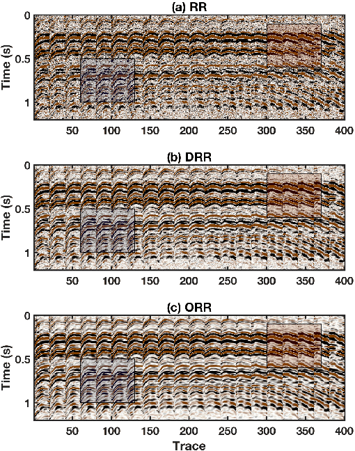
Figure 19. Real data example. (a) Reconstructed data using the RR method. (b) Reconstructed data using the DRR method. (c) Reconstructed data using the ORR method. In this case, $rank=20$. It is obvious that all three methods obtain dramatic improvement from the raw data. The ORR method obtains cleaner and spatially more coherent seismic events compared with other two methods.

field_dn_N12_z1
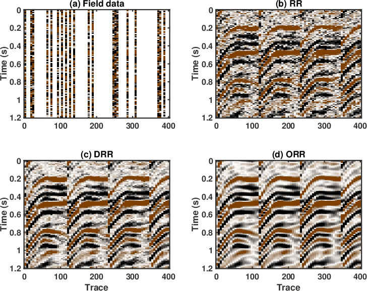
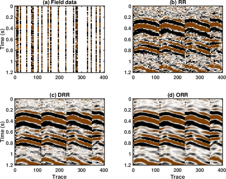
Figure 20. Zoomed comparison for the field data example (the blue frame box). (a) Incomplete data. (b) Reconstructed data using the RR method. (c) Reconstructed data using the DRR method. (d) Reconstructed data using the ORR method.

field_dn_N12_z2
Figure 21. Zoomed comparison for the field data example (the red frame box). (a) Incomplete data. (b) Reconstructed data using the RR method. (c) Reconstructed data using the DRR method. (d) Reconstructed data using the ORR method.

field_dn_N12_t80
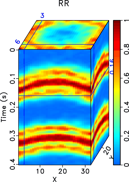
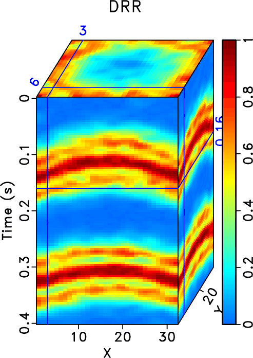
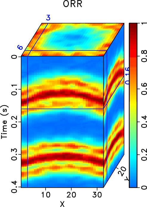
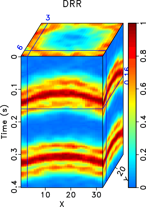
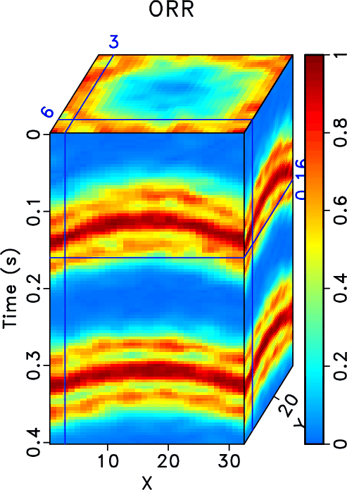
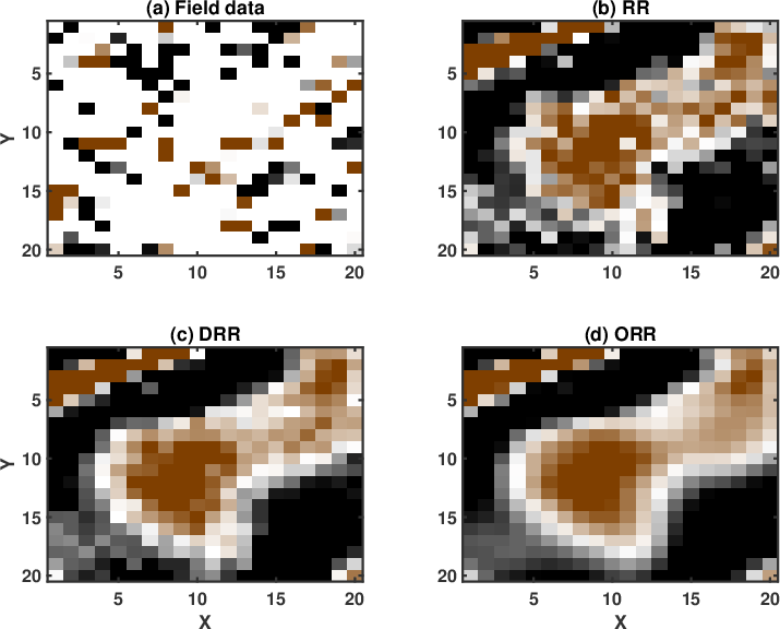
Figure 22. Comparison for constant time slice for the field data example ($t=0.32$s). (a) Incomplete data. (b) Reconstructed data using the RR method. (c) Reconstructed data using the DRR method. (d) Reconstructed data using the ORR method.

field_dn_N12_t160
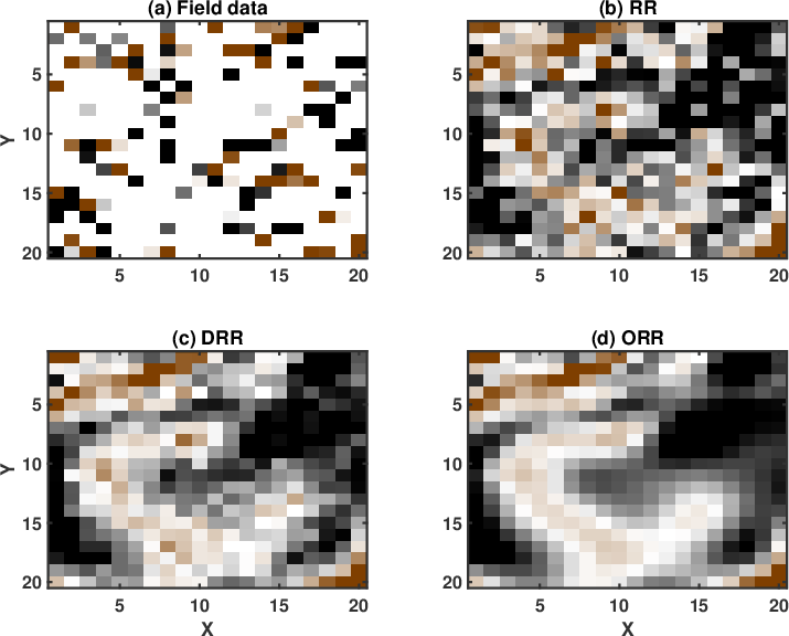
Figure 23. Comparison for constant time slice for the field data example ($t=0.64$s). (a) Incomplete data. (b) Reconstructed data using the RR method. (c) Reconstructed data using the DRR method. (d) Reconstructed data using the ORR method.

To test the sensitivities of each method to input noise level, we vary the variance of the additive random noise from 0.1 to 0.9 and calculate the output SNRs corresponding to different methods and draw the diagrams in Figure 12. The black line corresponds to the input SNR curve. The blue, red, and green lines correspond to the RR, DRR, and ORR methods, respectively. As the noise variance increases, the input SNR decreases, and so do the output SNRs of the three methods. However, the proposed method always outperforms the other two methods. It is worth noting that as the noise variance becomes larger, the differences between the proposed method and the other methods are also larger, which indicates that the proposed method is more effective for stronger noise.

To test the effectiveness of each method in situations with different sampling ratios, we vary the sampling ratio from 10% to 90%, and draw the input and output SNR curves in Figure 13. The colorful lines have the same meaning in this case. As we can see from Figure 13, the input SNR decreases with increasing sampling ratio. The output SNRs increase with increasing sampling ratios. It is clear that the output SNR curve of the proposed method is always above the other curves. The proposed method outperforms other two methods more when sampling ratio is higher.

To test the sensitivities of different methods to the input parameter, i.e., the predefined rank, we vary the rank from 4 to 15 and draw the SNR curves in Figure 14. Both RR and DRR methods decrease fast as the predefined rank increases while the SNR curve of the proposed ORR method is almost flat and is also above the other two curves. This test indicates that while the RR and DRR are more or less sensitive to the predefined rank, the proposed method is almost parameter-free, which makes the ORR method convenient to use in realistic situations.

To compare the computational cost of different methods, we measure the computing time for the synthetic example with linear events. The computation is done on a MacBook Pro laptop equipped with an Intel Core i7 CPU clocked at 2.5 GHz and 16 GB of RAM. The detailed computing time comparison is shown in Table 2. It shows that the computational cost of the ORR method is higher than the other two methods. The RR and DRR methods have almost the same computational cost while the proposed method costs 2-5 times more than the other two methods.

In order to test the effectiveness of the three methods on data containing curved events and to compare the performances of different methods in this case, we then use the second example to show the performance. Figure 15 shows the clean data, noisy data, and incomplete data with 70% traces randonly missing in a common midpoint gather. Figure 16 shows the reconstructed data using different methods. Because this dataset no longer meet the linear-event assumption of the rank-reduction based methods, we use a relatively higher rank in this example. The top row in Figure 16 shows results when $rank=12$. The bottom row in Figure 16 shows results when $rank=24$. It is clear that the three methods also work when there are curving events. The proposed method obtains obviously cleaner result than the other two methods. The SNRs of the incomplete data, data from the RR method, DRR method, and ORR method are 0.59, 14.11, 16.46, and 16.86 dB when $rank=12$ and are 0.59, 13.88, 16.01, and 16.83 dB when $rank=24$. We also calculate the local similarity between the exact solution shown in Figure 15a and each reconstructed data and show the similarity cubes in Figure 17. The local similarity corresponding to the proposed method is obviously higher than those from the other two methods, indicating a more accurate reconstruction result using the proposed method.

Finally, we apply the three methods to a 5D field data. We use the data previously used in Chen et al. (2016c). The data have been binned onto a regular grid and a common offset gather of the field data is shown in Figure 18. In Figure 18, the colored stripes are the recorded seismic traces. The white blanks denote the missing traces, which means that we do not observe seismic data in these positions. Because of the difficulty in displaying a 5D dataset, we only show a common midpoint gather here. The 3D common midpoint gather is rearranged into a 2D matrix for a better view. The two transparent colored windows denote two zooming areas for an amplified comparison. In this example, roughly 80% traces are missing from the regular grids. Because of the high ratio of missing traces, the observed seismic traces do not show any spatial coherency. It is difficult to see the waveforms from the raw data. The results from the three aforementioned methods are shown in Figure 19. After 5D reconstruction, the white blanks in the raw data have been filled with seismic traces. The waveforms become well aligned along the spatial direction. Compared with the raw data, all methods seem to obtain a dramatic improvement on the data quality. It is salient that both DRR and ORR methods obtain much smoother and cleaner results while the traditional RR method obtain a result that is noisier. Because of the strong residual noise in the result from the traditional RR method, the spatial coherency of the seismic events are deteriorated, which may affect the subsequent processing tasks like imaging, inversion, and interpretation. When zooming the data in the two transparent blue and red rectangles in both Figures 18 and 19, the comparison among different methods becomes much clearer. From Figures 20 and 21, we observe that although the DRR method obtain a much smoother result compared with the RR result, as already discussed from Chen et al. (2016c), the ORR method obtains a even smoother result, with energy spatially more correlative. We also extract two constant time slices at $t=0.32s$ and $t=0.64s$, respectively, and show them in Figures 22 and 23. The pixels corresponding to the proposed method are obviously smoother from the proposed method. The two reconstructed time slices from the proposed method show obvious shapes of a dome.

Table 1: SNRs comparison in dB for the synthetic example with linear events.

	Incomplete	RR	DRR	ORR
N=3	-4.59	9.96	11.68	12.03
N=5	-4.59	8.01	10.87	11.99
N=10	-4.59	5.51	9.54	11.83

Table 2: Computing time comparison in seconds for the synthetic example with linear events. The computation is done on a MacBook Pro laptop equipped with an Intel Core i7 CPU clocked at 2.5 GHz and 16 GB of RAM.

	RR	DRR	ORR
N=3	246.39	249.63	656.33
N=5	249.37	252.52	923.45
N=10	250.28	255.27	1226.63

Table 3: SNRs comparison in dB for the synthetic example with hyperbolic events.

	Incomplete	RR	DRR	ORR
N=12	0.59	14.11	16.46	16.86
N=24	0.59	13.88	16.01	16.83