|
 |
 |
 | Seismic data interpolation using streaming prediction filter in the frequency domain |  |
![[pdf]](icons/pdf.png) |
Next: - - streaming prediction
Up: Theory
Previous: Two-step interpolation strategy
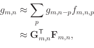
In the  -
- domain, the PF predicts the data along the spatial
direction, and the relationship between data and prediction filter can
be summarized as
domain, the PF predicts the data along the spatial
direction, and the relationship between data and prediction filter can
be summarized as
where  and
and  are the indices of the seismic data sample
  along the frequency
axis and space
axis, respectively. Vector
along the frequency
axis and space
axis, respectively. Vector
 is the group of filter coefficients
  in
the adaptive prediction filter, and each group
corresponds to a data sample
. Vector
in
the adaptive prediction filter, and each group
corresponds to a data sample
. Vector
 denotes several data points
  with spatial shift
  near
. Spatial shift
is related to the filter size (the
number of filter coefficients in
), and the filter
size should theoretically be larger than or equal to the number of
seismic events contained in the local space window. When the causal
filter structure is considered, as shown in Fig. 1a,
the spatial shift is chosen as
near
. Spatial shift
is related to the filter size (the
number of filter coefficients in
), and the filter
size should theoretically be larger than or equal to the number of
seismic events contained in the local space window. When the causal
filter structure is considered, as shown in Fig. 1a,
the spatial shift is chosen as
![$ p \in [1, 3] $](img35.png) , vector
can be expressed as
, vector
can be expressed as
 , and
, and
 . For the non-causal filter
structure (Fig. 1b), the spatial shift is
. For the non-causal filter
structure (Fig. 1b), the spatial shift is
![$ p \in
[-3,-1] \cup [1, 3] $](img38.png) , and vector
and
can be represented as
, and vector
and
can be represented as
 ,
,
 .
.
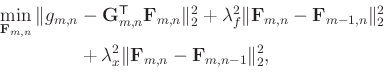
With Eq. (3), we established the following minimization
problem, like Eq. (1), to calculate filter
:
 |
(4) |
According to the above explanation of vector
, there
are several unknown filter coefficients, yet we established only one
equation. Eq. (4) describes an ill-posed problem,
which requires constraints to obtain a stable solution. The framework
of the streaming computation (Fomel and Claerbout, 2016; Sacchi and Naghizadeh, 2009; Liu and Li, 2018)
establishes the constraint relationship by using local smoothness. We
extended this method into the frequency domain, including the
-
domain and the
-
- domain (the next section) to stabilize the
filter coefficient solution. Additionally, we discussed in detail the
effects of filter structure and processing path, and provided the
corresponding interpolation algorithms. Here, multiple constraints
based on local smoothness are used to constrain the solution of
Eq. (4):
domain (the next section) to stabilize the
filter coefficient solution. Additionally, we discussed in detail the
effects of filter structure and processing path, and provided the
corresponding interpolation algorithms. Here, multiple constraints
based on local smoothness are used to constrain the solution of
Eq. (4):
where
 and
and
 are the weights of the
regularization terms along the frequency
and space
axes.
are the weights of the
regularization terms along the frequency
and space
axes.
 shows the local smoothness along the frequency direction
(
shows the local smoothness along the frequency direction
(
 ). Likewise,
 controls the local smoothness along
the space direction as
controls the local smoothness along
the space direction as
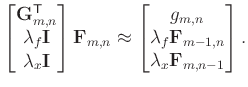
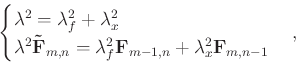
 . The block matrix
Eq. (6) has the same solution as
Eq. (5), and it demonstrates the effect of the local
smoothness constraints; when
. The block matrix
Eq. (6) has the same solution as
Eq. (5), and it demonstrates the effect of the local
smoothness constraints; when
 and
and
 are considered known, the local smoothness
conditions (
and
), as newly added equations,
can be used to stabilize the solution of
:
are considered known, the local smoothness
conditions (
and
), as newly added equations,
can be used to stabilize the solution of
:
 |
(6) |
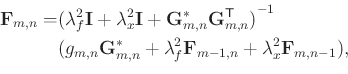
One can obtain the following least-squares solution of
Eq. (5) and (6):
where
 denotes the conjugate operator. Let
 |
(8) |
we get a simplified equation:
 |
(9) |
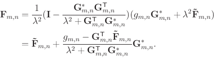
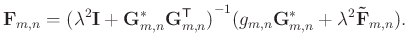
Meanwhile,
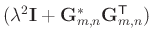 has the
analytical inversion
has the
analytical inversion
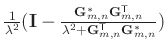 when one
extends the Sherman-Morrison formula (Sherman and Morrison, 1950; Hager, 1989; Bartlett, 1951) to the complex space. We can obtain the analytical solution
of the
-
SPF:
when one
extends the Sherman-Morrison formula (Sherman and Morrison, 1950; Hager, 1989; Bartlett, 1951) to the complex space. We can obtain the analytical solution
of the
-
SPF:
Eq. (10) shows a recursive relationship from the
previous filters (
and
) to
current filter
. For data interpolation,
Eq. (2) becomes a well-posed problem, and the unknown
data sample can be calculated by
 |
(11) |
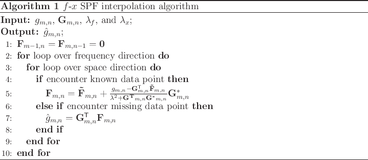
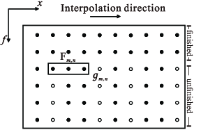
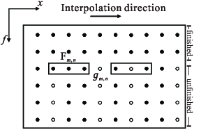
In 2D data interpolation, we proposed the following
Algorithm 1 to reconstruct the missing seismic data
by using the 2D
-
SPF. To start,
and
are initialized to
 . When the
processing path in Algorithm 1 is followed, both
and
are known. We designed
a space-causal filter form (Fig. 1a) for the
-
SPF. Fig. 1b suggests that the space-noncausal form
may involve the interference of the unknown data samples, but the
causal one can avoid this problem.
. When the
processing path in Algorithm 1 is followed, both
and
are known. We designed
a space-causal filter form (Fig. 1a) for the
-
SPF. Fig. 1b suggests that the space-noncausal form
may involve the interference of the unknown data samples, but the
causal one can avoid this problem.
|
|---|
causal2d,noncausal2d
Figure 1. Space-causal filter form (a) and space-noncausal filter form (b)
in the
-
domain. Solid circle denotes known sample,
and hollow circle denotes unknown sample.
|
|---|
![[png]](icons/viewmag.png) ![[scons]](icons/configure.png)
|
|---|
|
|
|
|
| Seismic data interpolation using streaming prediction filter in the frequency domain | |
|
Next: - - streaming prediction
Up: Theory
Previous: Two-step interpolation strategy
2022-04-15