|
|
|
|
Seismic data interpolation using streaming prediction filter in the frequency domain |
The extension to the 3D ![]() -
-![]() -
-![]() domain is straightforward as the
domain is straightforward as the
![]() -
-![]() -
-![]() SPF can also efficiently perform data interpolation in
high dimensions. In the
SPF can also efficiently perform data interpolation in
high dimensions. In the ![]() -
-![]() -
-![]() domain, the prediction
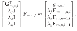
relationship for seismic data in a certain frequency slice is
expressed as
domain, the prediction
relationship for seismic data in a certain frequency slice is
expressed as
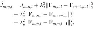
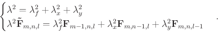
The cost function is defined as
 |
(17) |
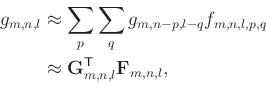
Furthermore, the unknown data sample in the 3D data cube can be calculated as
Because the ![]() -
-![]() -
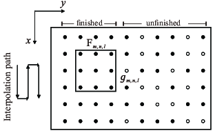
-![]() SPF predicts data along two spatial
directions, we defined a new processing path in the space plane with
zigzag shape (Fig. 2a) to prevent unnecessary filter
initialization. Meanwhile, the
SPF predicts data along two spatial
directions, we defined a new processing path in the space plane with
zigzag shape (Fig. 2a) to prevent unnecessary filter
initialization. Meanwhile, the ![]() -
-![]() -
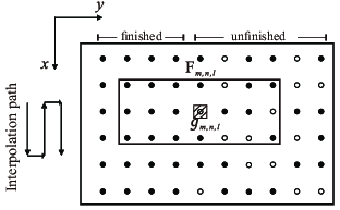
-![]() SPF was assigned to the
proposed filter form (Fig. 2a), which can better
reduce the influence of unknown data samples than the noncausal filter
in spatial directions (Fig. 2b). Following the
processing path of Algorithm 2 for data processing,
SPF was assigned to the
proposed filter form (Fig. 2a), which can better
reduce the influence of unknown data samples than the noncausal filter
in spatial directions (Fig. 2b). Following the
processing path of Algorithm 2 for data processing,
![]() ,
,
![]() , and
, and
![]() can be seen as known, requiring only
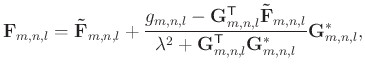
calculating Eq. (16) and (18) to
obtain the results.
can be seen as known, requiring only
calculating Eq. (16) and (18) to
obtain the results.
|
|---|
|
causal3d,noncausal3d
Figure 2. Proposed filter form (a) and space-noncausal filter form (b) in the |
|
|
|
|
|
|
Seismic data interpolation using streaming prediction filter in the frequency domain |