Time-to-depth conversion and seismic velocity estimation using time-migration velocity

Finite difference method

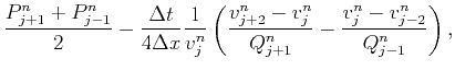
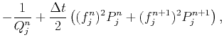
This method was inspired by the Lax-Friedrichs method for hyperbolic conservation laws Lax (1954) due to its total variation diminishing property. We use the ``Lax-Friedrichs averaging'' and the wide 5-point stencil in space. The scheme is given by

$$P^{n+1}_j = \frac{P_{j+1}^n+P_{j-1}^n}{2} -\frac{\Delta t}{4\Delta x} \frac{1... ...(\frac{v^n_{j+2}-v^n_j}{Q^n_{j+1}}- \frac{v^n_{j}-v^n_{j-2}}{Q^n_{j-1}}\right),$$ (21)

$$-\frac{1}{Q^{n+1}_j} = -\frac{1}{Q^n_j}+ \frac{\Delta t}{2}\left((f_j^n)^2P_j^n+(f_j^{n+1})^2P_j^{n+1}\right),$$ (22)

where $v\equiv fQ$ . We impose the following boundary conditions $Q^n_0=Q^n_{nx-1}=1$ , $P_0^n=P^n_{nx-1}=0$ corresponding the straight boundary rays. We set the initial conditions $Q_j^0=1$ , $P^0_j=0$ corresponding to the initial conditions for the image rays traced backward: $Q=1$ , $P=0$ .