|
|
|
|
A parallel sweeping preconditioner for heterogeneous 3D Helmholtz equations |
Since a subtree-to-subteam mapping will assign each supernode of an
auxiliary problem to a team of processes, and each panel of the original
3D domain is by construction a subset of the domain of an auxiliary
problem, it is straightforward to extend the supernodal subteam assignments to
the full domain. We should then be able to distribute global vectors so
that no communication is required for readying panel subvectors for
subdomain solves (via extension by zero for interior panels, and trivially for
the first panel). Since our nested dissection process does not partition in
the shallow dimension of quasi-2D subdomains (see Fig. 3),
extending a vector defined over a panel of the original domain onto the
PML-padded auxiliary domain simply requires individually extending each
supernodal subvector by zero in the ![]() direction.
direction.
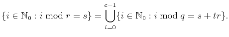
Consider an element-wise two-dimensional cyclic distribution
(30) of a frontal matrix ![]() over
over ![]() processes using an
processes using an
![]() process grid, where
process grid, where ![]() and
and ![]() are
are
![]() . Then the
. Then the
![]() entry will be stored by the process in the
entry will be stored by the process in the
![]() position in the process grid.
Using the notation from (30), this distributed front would
be denoted as
position in the process grid.
Using the notation from (30), this distributed front would
be denoted as
![]() , while its top-left quadrant would be referred to
as
, while its top-left quadrant would be referred to
as
![]() (see Fig. 5 for a depiction of an
(see Fig. 5 for a depiction of an ![]() matrix distribution).
matrix distribution).
 |
Loosely speaking, ![]() means that each column
of
means that each column
of ![]() is distributed using the scheme denoted by
is distributed using the scheme denoted by ![]() , and each row
is distributed using the scheme denoted by
, and each row
is distributed using the scheme denoted by ![]() . For the element-wise
two-dimensional distribution used for
. For the element-wise
two-dimensional distribution used for ![]() ,
, ![]() , we have that the
columns of
, we have that the
columns of ![]() are distributed like Matrix Columns (
are distributed like Matrix Columns (![]() ), and the rows
of
), and the rows
of ![]() are distributed like Matrix Rows (
are distributed like Matrix Rows (![]() ). While this notation may seem
vapid when only working with a single distributed matrix, it is useful when
working with products of distributed matrices. For instance, if a `
). While this notation may seem
vapid when only working with a single distributed matrix, it is useful when
working with products of distributed matrices. For instance, if a `![]() ' is
used to represent rows/columns being redundantly stored (i.e., not distributed),
then the result of every process multiplying its local submatrix of
' is
used to represent rows/columns being redundantly stored (i.e., not distributed),
then the result of every process multiplying its local submatrix of
![]() with its local submatrix of
with its local submatrix of
![]() forms a distributed
matrix
forms a distributed
matrix
![]() , where the last
expression refers to the local multiplication process.
, where the last
expression refers to the local multiplication process.
We can now decide on a distribution for each supernodal subvector, say
![]() , based on the criteria that it should be fast to
form
, based on the criteria that it should be fast to
form
![]() and
and
![]() in the same
distribution as
in the same
distribution as
![]() , given that
, given that ![]() is distributed as
is distributed as
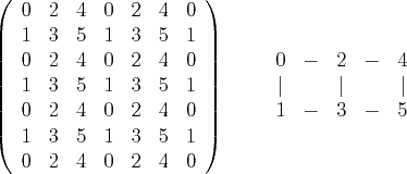
![]() . Suppose that we define a Column-major Vector distribution
(
. Suppose that we define a Column-major Vector distribution
(![]() ) of
) of
![]() , say
, say
![]() , to
mean that entry
, to
mean that entry ![]() is owned by process
is owned by process ![]() , which corresponds
to position
, which corresponds
to position
![]() in the process grid
(if the grid is constructed with a column-major ordering of the process ranks;
see the left side of Fig. 6).
Then a call to
in the process grid
(if the grid is constructed with a column-major ordering of the process ranks;
see the left side of Fig. 6).
Then a call to MPI_Allgather (10) within each row of the
process grid would allow for each process to collect all of the data necessary
to form
![]() , as for any process row index
, as for any process row index
![]() ,
,
 |
 |
Similarly, if
![]() was distributed with a Row-major Vector
distribution (
was distributed with a Row-major Vector
distribution (![]() ), as shown on the right side of Fig. 6,
say
), as shown on the right side of Fig. 6,
say
![]() , so that
entry
, so that
entry ![]() is owned by the process in position
is owned by the process in position
![]() of the process grid, then a call to
of the process grid, then a call to
MPI_Allgather within each column of the process grid would provide
each process with the data necessary to form
![]() .
Under reasonable assumptions, both of these redistributions can be shown to
have per-process communication volume lower bounds of
.
Under reasonable assumptions, both of these redistributions can be shown to
have per-process communication volume lower bounds of
![]() (if
(if ![]() is
is
![]() ) and latency lower bounds of
) and latency lower bounds of
![]() (9).
We also note that translating between
(9).
We also note that translating between
![]() and
and
![]() simply requires permuting which process owns each
local subvector, so the communication volume would be
simply requires permuting which process owns each
local subvector, so the communication volume would be ![]() ,
while the latency cost is
,
while the latency cost is ![]() .
.
We have thus described efficient techniques for redistributing
![]() to both the
to both the
![]() and
and
![]() distributions, which are the first steps
for our parallel algorithms for forming
distributions, which are the first steps
for our parallel algorithms for forming
![]() and
and
![]() , respectively: Denoting the distributed result of
each process in process column
, respectively: Denoting the distributed result of
each process in process column
![]() multiplying its local
submatrix of
multiplying its local
submatrix of
![]() by its local subvector of
by its local subvector of
![]() as
as
![]() , it holds that
, it holds that
![]() .
Since Eq. (7) also implies that each process's local data
from a
.
Since Eq. (7) also implies that each process's local data
from a
![]() distribution is a subset of its local data from a
distribution is a subset of its local data from a
![]() distribution, a simultaneous summation and scattering of
distribution, a simultaneous summation and scattering of
![]() within process rows, perhaps via
within process rows, perhaps via
MPI_Reduce_scatter or MPI_Reduce_scatter_block, yields the
desired result,
![]() . An analogous process
with
. An analogous process
with
![]() and
and
![]() yields
yields
![]() , which can then be cheaply
permuted to form
, which can then be cheaply
permuted to form
![]() . Both calls to
. Both calls to
MPI_Reduce_scatter_block can be shown to have the same communication
lower bounds as the previously discussed MPI_Allgather
calls (9).
As discussed at the beginning of this section, defining the distribution of
each supernodal subvector specifies a distribution for a global vector,
say
![]() . While the
. While the
![]() distribution shown in
the left half of Fig. 6 simply assigns entry
distribution shown in
the left half of Fig. 6 simply assigns entry ![]() of a
supernodal subvector
of a
supernodal subvector
![]() , distributed over
, distributed over ![]() processes, to
process
processes, to
process ![]() , we can instead choose an alignment
parameter,
, we can instead choose an alignment
parameter, ![]() , where
, where
![]() , and assign entry
, and assign entry ![]() to
process
to
process
![]() . If we simply set
. If we simply set ![]() for every
supernode, as the discussion at the beginning of this subsection implied, then
at most
for every
supernode, as the discussion at the beginning of this subsection implied, then
at most
![]() processes will store data for the root separator
supernodes of a global vector, as each root separator only has
processes will store data for the root separator
supernodes of a global vector, as each root separator only has
![]() degrees of freedom by construction.
However, there are
degrees of freedom by construction.
However, there are
![]() root separators, so we can easily allow
for up to
root separators, so we can easily allow
for up to ![]() processes to share the storage of a global vector if the
alignments are carefully chosen.
It is important to notice that the top-left quadrants of the
frontal matrices for the root separators can each be distributed over
processes to share the storage of a global vector if the
alignments are carefully chosen.
It is important to notice that the top-left quadrants of the
frontal matrices for the root separators can each be distributed over
![]() processes, so
processes, so
![]() processes can actively
participate in the corresponding triangular matrix-vector multiplications.
processes can actively
participate in the corresponding triangular matrix-vector multiplications.
|
|
|
|
A parallel sweeping preconditioner for heterogeneous 3D Helmholtz equations |