|
|
|
|
Least-squares path-summation diffraction imaging using sparsity constraints |
Next: Discussion Up: Merzlikin et al.: Least-squares Previous: Synthetic data example
|
|
|
|
Least-squares path-summation diffraction imaging using sparsity constraints |
We apply the proposed approach to the Viking Graben dataset (Keys and Foster, 1998). Klokov and Fomel (2012a) previously performed diffraction imaging of the Viking Graben dataset using Hybrid Radon transform in the dip-angle common image gathers' domain. Gonzalez et al. (2016) perform diffraction-based depth velocity analysis on the dataset.
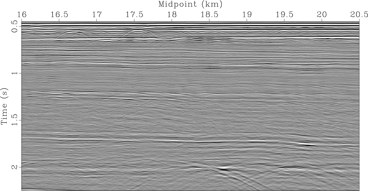
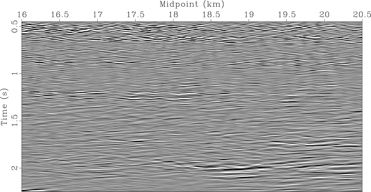
Figure 10a illustrates the zero-offset section. It can be noticed that gradually dipping continuous reflections are interrupted by faults encoded in the diffracted wavefield. Additional diffractions are associated with rough reflector surfaces. Diffractions exhibit significantly lower amplitudes than reflections, and a separation procedure aimed to emphasize diffractions must be applied before proceeding along the workflow. We separated diffractions (Figure 10b) from reflections using PWD filter (Fomel et al., 2007) and first imaged them using conventional post-stack Kirchhoff time migration (Figure 11b). Shallow high-diffractivity layer can be noticed in the upper part of the image. Fault surfaces and diffractivity associated with reflector roughness stand out in comparison with conventional migration image shown in Figure 11a. However, because of the overlap of diffraction responses and the presence of noise, the parts of the image between faults are hard to interpret.

|
|---|
|
dmo-w,pwd-w
Figure 10. (a) Dip-moveout (DMO) stack; (b) plane-wave destruction filter (PWD, |
|
|


|
|---|
|
image-fw,conv-image-pwd
Figure 11. Conventional Kirchhoff migration applied to DMO and PWD stacks (Figures 10a and 10b) |
|
|
We apply the “chain" of operators inversion approach to improve diffraction signal-to-noise ratio
and increase the diffraction image reliability.
First, we prepare the data to be fit by the inversion (equation 6). The zero-offset section after application
of
PWD in the data domain (
![]() ) followed by path-summation integral filter (
) followed by path-summation integral filter (
![]() )
is shown in Figure 12a. These are the data to be fit, which
can be treated as diffraction probability. Slope values required for PWD in the data domain (
)
is shown in Figure 12a. These are the data to be fit, which
can be treated as diffraction probability. Slope values required for PWD in the data domain (
![]() )
and for shaping regularization in the model space (
)
and for shaping regularization in the model space (
![]() ) are estimated using zero-offset section (Figure 10a) and conventional Kirchhoff
migration image (Figure 11a) correspondingly. We run
) are estimated using zero-offset section (Figure 10a) and conventional Kirchhoff
migration image (Figure 11a) correspondingly. We run ![]() outer iterations and
outer iterations and ![]() inner to restore reflectivity
and diffractivity shown in Figure 12. It can be seen that
diffractions are significantly more highlighted than in the Kirchhoff migration image of the section after PWD (Figure 11b) and appear to be denoised.
At the same time, crosstalk between reflections and diffractions is strong and a lot of strong reflection energy is in the null space of the operator. For instance,
compare reflectivity restored (Figure 12b) with conventional Kirchhoff image (Figure 11a) at small TWTT, e.g.
inner to restore reflectivity
and diffractivity shown in Figure 12. It can be seen that
diffractions are significantly more highlighted than in the Kirchhoff migration image of the section after PWD (Figure 11b) and appear to be denoised.
At the same time, crosstalk between reflections and diffractions is strong and a lot of strong reflection energy is in the null space of the operator. For instance,
compare reflectivity restored (Figure 12b) with conventional Kirchhoff image (Figure 11a) at small TWTT, e.g.
![]() .
For reflection-diffraction crosstalk, for instance, refer to the fragment delimited by
.
For reflection-diffraction crosstalk, for instance, refer to the fragment delimited by
![]() TWTT and
TWTT and
![]() distance. Continuous layering
associated with reflections leaks to the diffraction image domain and overlaps with discontinuities along the faults. Events with similar
behavior correspond to
unconformities at around
distance. Continuous layering
associated with reflections leaks to the diffraction image domain and overlaps with discontinuities along the faults. Events with similar
behavior correspond to
unconformities at around ![]() TWTT between
TWTT between
![]() distance.
distance.


|
|---|
|
pi-pwd,reflectivity-with-pwd,diffractivity-with-pwd
Figure 12. (a) DMO section (Figure 10a) weighted by path-summation integral operator ( |
|
|
To address the null space and crosstalk problems we generate the data for the second inversion (equation 8), invert for reflections and diffractions
(we run ![]() outer iterations and
outer iterations and ![]() inner) and produce the models shown in Figure 13.
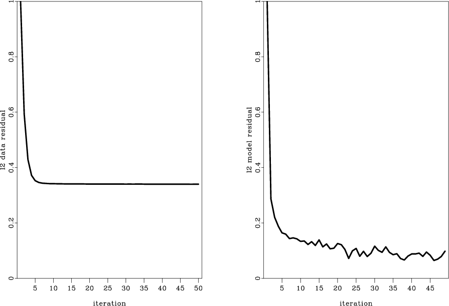
Orthogonalization of the diffraction update is shown in Figure 14. Convergence curves are shown in Figure 15.
It can be seen that reflections are recovered from the null space (refer to the shallow events) and crosstalk between diffractions and
reflections has also been reduced. In particular continuous layering events delimited by
inner) and produce the models shown in Figure 13.
Orthogonalization of the diffraction update is shown in Figure 14. Convergence curves are shown in Figure 15.
It can be seen that reflections are recovered from the null space (refer to the shallow events) and crosstalk between diffractions and
reflections has also been reduced. In particular continuous layering events delimited by
![]() TWTT and
TWTT and
![]() distance
and around
distance
and around ![]() TWTT between
TWTT between
![]() distance are suppressed. There is still a remainder
of events with elongated shapes in diffraction image (Figure 13c). These events can be connected with rough surface features,
which are too irregular to be described by the chosen smoothing radius in shaping regularization penalizing reflections.
Less aggressive smoothing and more detailed dip field in the model space should allow moving these events back to the reflection image domain.
Stronger thresholding can also help.
distance are suppressed. There is still a remainder
of events with elongated shapes in diffraction image (Figure 13c). These events can be connected with rough surface features,
which are too irregular to be described by the chosen smoothing radius in shaping regularization penalizing reflections.
Less aggressive smoothing and more detailed dip field in the model space should allow moving these events back to the reflection image domain.
Stronger thresholding can also help.


|
|---|
|
pi-no-pwd,reflectivity-no-pwd,diffractivity-no-pwd
Figure 13. (a) DMO section (Figure 10a) weighted by path-summation integral operator ( |
|
|


|
|---|
|
update-b4-refl,update-a4-diffr
Figure 14. Updates to the model: (a) update to diffractions before orthogonalization (equation 12; reflections have the same update); (b) update to diffractions after orthogonalization: reflections are suppressed and diffraction-related update is more visible. |
|
|
|
|---|
|
convergence
Figure 15. Convergence of the inversion with no PWD (equation 8): left - residual in the data space; right - difference between consecutive models. |
|
|
Finally we restore high wavenumbers and model reflections (Figure 16a) and diffractions (Figure 16b). As in the synthetic data example, diffractions in wavenumber restoration inversion are additionally penalized by the locations' mask determined from the output of the second inversion cascade (Figure 13c). We then subtract their sum from the zero-offset DMO section (Figure 10a) and arrive at the following noise estimate (Figure 16c). Noise section is plotted with the same gain as the “restored" diffractions. Signal and noise orthogonalization (Chen and Fomel, 2015) is applied to account for aperture difference between observed (Figure 10b) and restored diffractions (Figure 16b) (for instance, often only a single diffraction flank can be observed in the data leading to spuriously high difference or the “noise estimate”) and to bring back some of the energy accidentally leaked to the noise domain (Figure 16c). Some residuals can be noticed in the lower part of the noise section, which can have a signature intermediate between reflections and diffractions, were not attributed to either. Upper part of the noise section exhibits low magnitude residuals stating high accuracy of the method. Besides that, restored diffractions (Figure 16b) exhibit high correlation with PWD section (Figure 10b) also supporting high efficiency of the method.


|
|---|
|
reflections-restored,diffraction-restored,noise-restored-orthogon
Figure 16. (a) “Restored" reflections; (b) “restored" diffractions; (c) “restored" noise - (a) and (b) subtracted from the DMO section (Figure 10a). |
|
|
Overall impression of the image shown in Figure 13c can be contradictory because of the continuity loss. However,
diffractions have spiky and intermittent distribution, which correlates well with the faults and other discontinuities observed in the conventional image (Figure 11a).
To highlight this statement we overlay the conventional image (Figure 11a) with estimated diffractivity (Figure 17).
High correlation between continuous layering interruptions and diffractions can be observed (e.g.
![]() TWTT and
TWTT and
![]() ).
Moreover, smaller scale faults, which are not evident from the “conventional" image, are highlighted and denoised with the help of the approach
proposed. For instance, refer to the fragment delimited by
).
Moreover, smaller scale faults, which are not evident from the “conventional" image, are highlighted and denoised with the help of the approach
proposed. For instance, refer to the fragment delimited by
![]() TWTT and
TWTT and
![]() distance. Some faults are not pronounced
in the diffraction image. On the other hand, the approach allows increasing the confidence of the diffractions present in the image and distinguishing
them from noise. In other words, even though some events might be lost, we can be confident in the events that were successfully imaged.
distance. Some faults are not pronounced
in the diffraction image. On the other hand, the approach allows increasing the confidence of the diffractions present in the image and distinguishing
them from noise. In other words, even though some events might be lost, we can be confident in the events that were successfully imaged.

|
|---|
|
combined
Figure 17. Diffractivity estimated overlaid on top of the conventional image (Figure 11a). |
|
|
|
|
|
|
Least-squares path-summation diffraction imaging using sparsity constraints |