Noncausal $f$ -$x$ -$y$ regularized nonstationary prediction filtering for random noise attenuation on 3D seismic data

The review of $f$ -$x$ NRNA

Seismic section $S(t,x)$ in $f$ -$x$ domain is predictable if it only includes linear events in $t-x$ domain. The relationship between the n-th trace and (n-i)-th trace can be easily described as

$${{S}_{n}}(f)=\sum\limits_{i=1}^{M}{{{a}_{i}}(f){{S}_{n-i}}(f)},$$ (1)

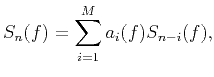
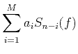
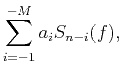
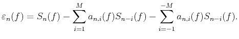
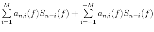
where M is the number of events in 2D seismic section. Eq. (1) describes forward prediction equations, namely causal prediction filtering equations (Gulunay, 2000). In the case of both forward and backward prediction equations (noncausal prediction filter), Eq. 1 can be written as (Spitz, 1991; Gulunay, 2000; Naghizadeh and Sacchi, 2009; Liu et al., 1991)

$${{S}_{n}}(f) \sum\limits_{i=1}^{M}{{{a}_{i}}{{S}_{n-i}}}(f) \sum\limits_{i=-1}^{-M}{{{a}_{i}}{{S}_{n-i}}(f)},$$ (2)

where M is the parameter related to the number of events. Note that Eq. 2 implies the assumption $\sum\nolimits_{i=1}^{M}{{{a}_{i}}{{S}_{n-i}}(f)}$=0$.$5${{S}_{n}}(f)$ and $\sum\nolimits_{i=-1}^{-M}{{{a}_{i}}{{S}_{n-i}}(f)}$=0$.$5${{S}_{n}}(f)$ . Theoretically, ${{a}_{i}}$ in forward prediction equations is the complex conjugation of ${{a}_{-i}}$ in backward equations (Galbraith, 1984). Gulunay (2000) pointed that it is possible to reduce the order of the normal equations from 2M to M because the coefficients of noncausal prediction filter have conjugate symmetry. f-x prediction filtering has the assumption that the events of seismic section are linear. If seismic events are not linear, or the amplitudes of wavelet are varying, they no longer follow linear or stationary assumptions (Canales, 1984). One needs to perform $f$ -$x$ prediction filtering over a short sliding window in time and space to cope with continuous changes in dips (Naghizadeh and Sacchi, 2009). Fomel (2009) developed a general method of RNA using shaping regularization technology, which is implemented for real number. Liu et al. (1991) extended the RNA method to $f$ -$x$ domain for complex numbers and applied it to seismic random noise attenuation for 2D seismic data. The $f$ -$x$ NRNA is defined as (Liu et al., 1991)

$${{\varepsilon }_{n}}(f)={{S}_{n}}(f)-\sum\limits_{i=1}^{M}{{{a}_{n,i}}(f){{S}_{n-i}}(f)}-\sum\limits_{i=-1}^{-M}{{{a}_{n,i}}(f){{S}_{n-i}}(f)}.$$ (3)

Eq. 3 indicates that one trace noise-free in $f$ -$x$ domain can be predicted by adjacent traces with the different weights ${{a}_{n,i}}(f)$ . Note that the weights ${{a}_{n,i}}(f)$ is varying along the space direction, which indicated by subscript i in ${{a}_{n,i}}(f)$ . In Eq. 3, the coefficients $a$ is the function of space i, but it is not in Eq. 2. When applying $f$ -$x$ NRNA to seismic noise attenuation, we assume the prediction error ${{\varepsilon }_{n}}(f)$ is the random noise and the predictable part $\sum\limits_{i=1}^{M}{{{a}_{n,i}}(f){{S}_{n-i}}(f)}+\sum\limits_{i=-1}^{-M}{{{a}_{n,i}}(f){{S}_{n-i}}(f)}$ is the signal. Finding spatial-varying coefficients ${{a}_{n,i}}(f)$ form Eq. 3 is ill-posed problem because there are more unknown variables than constraint equations. To obtain the coefficients, we should add constraint equations. Shaping regularization (Fomel, 2009) can be used to solve the under-constrained problem (Liu et al., 1991). The RNA method can also be used for seismic data processing in t-x-y domain, such as seismic data interpolation (Liu and Fomel, 2011).

Noncausal $f$ -$x$ -$y$ regularized nonstationary prediction filtering for random noise attenuation on 3D seismic data