Wide-azimuth angle gathers for wave-equation migration

Moveout function

In this section, we derive the formula for the moveout function characterizing reflections in the extended $\{ {\boldsymbol{\lambda}} ,\tau \}$ domain. The purpose of this derivation is to find a procedure for angle decomposition, i.e. a representation of reflectivity as a function of reflection and azimuth angles.

An implicit assumption made by all methods of angle decomposition is that we can describe the reflection process by locally planar objects. Such methods assume that (locally) the reflector is a plane, and that the incident and reflected wavefields are also (locally) planar. Only with these assumptions we can define vectors in-between which we measure angles like the angles of incidence and reflection, as well as the azimuth angle of the reflection plane. Our method uses this assumption explicitly. However, we do not assume that the wavefronts are planar. Instead, we consider each (complex) wavefront as a superposition of planes with different orientations. In the following, we discuss how each one of these planes would behave during the extended imaging and angle decomposition. Thus, our method applies equally well for simple and complex wavefields characterized by multipathing.

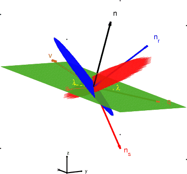
We define the following unit vectors to describe the reflection geometry and the conventional and extended imaging conditions:

• ${\bf n}$ : a unit vector aligned with the reflector normal;
• ${\bf a}$ : a unit vector representing the projection of the azimuth vector ${\bf v}$ in the reflector plane;
• ${\bf n}_s$ : a unit vector orthogonal to the source wavefront;
• ${\bf n}_r$ : a unit vector orthogonal to the receiver wavefront;
• ${\bf q}$ : a unit vector at the intersection of the reflection plane and the reflector plane.

By construction, vectors ${\bf n}$ , ${\bf n}_s$ , ${\bf n}_r$ and ${\bf q}$ are co-planar and vectors ${\bf n}$ and ${\bf q}$ are orthogonal, Figure 1.

With these definitions, the (planar) source and receiver wavefields are given by the expressions:

$${\bf n}_s\cdot {\bf x} = v t_s\;,$$ (6)

$${\bf n}_r\cdot {\bf x} = v t_r\;.$$ (7)

Here, ${\bf x}$ are space coordinates, $t_s$ and $t_r$ are times defining the planes under consideration, and $v$ represents velocity. Equations 6 and 7 define the conventional imaging condition given by equations 1 and 2. This condition states that an image is formed when the source and receiver wavefields are time-coincident at reflection points. In Equations 6 and 7, we explicitly impose the condition that the source and receiver planes and the reflector plane intersect at the image point.

Similarly, we can rewrite the extended imaging condition using the planar approximation of the source and receiver wavefields using the expressions:

$${\bf n}_s\cdot \left ({\bf x}- {\boldsymbol{\lambda}} \right) = v \left (t_s - \tau \right)\;,$$ (8)

$${\bf n}_r\cdot \left ({\bf x}+ {\boldsymbol{\lambda}} \right) = v \left (t_r + \tau \right)\;.$$ (9)

As discussed earlier, ${\boldsymbol {\lambda }}$ and $\tau$ are space- and time-lags, and $v$ represents the local velocity at the image point, assumed to be constant in the immediate vicinity of this point. This assumption is justified by the need to operate with planar objects, as indicated earlier. With this construction, the source and receiver planes are shifted relative to one-another by equal quantities in the positive and negative directions and in space and time, equations 3-4.

We can eliminate the space variable ${\bf x}$ by substituting equation 6 in equation 8 and equation 7 in equation 9:

$${\bf n}_s\cdot {\boldsymbol{\lambda}} = v \tau\;,$$ (10)

$${\bf n}_r\cdot {\boldsymbol{\lambda}} = v \tau\;.$$ (11)

Furthermore, we can re-arrange the system given by equations 10 and 11 by sum and difference of the equations:

$$\left ({\bf n}_s+ {\bf n}_r\right)\cdot {\boldsymbol{\lambda}} = 2 v \tau\;,$$ (12)

$$\left ({\bf n}_s- {\bf n}_r\right)\cdot {\boldsymbol{\lambda}} = 0\;.$$ (13)

So far, we have not assumed any relation between the vectors characterizing the source and receiver planes, ${\bf n}_s$ and ${\bf n}_r$ . However, if the source and receiver wavefields correspond to a reflection from a planar interface, these vectors are not independent of one-another, but are related by Snell's law which can be formulated as

$${\bf n}_r= {\bf n}_s- 2\left ({\bf n}_s\cdot {\bf n}\right){\bf n}\;.$$ (14)

This relations follows from geometrical considerations and it is based on the conservation of ray vector projection along the reflector. Equation 14 is only valid for PP reflections in an isotropic medium.

Substituting Snell's law into the system 12-13, and after trivial manipulations of the equations, we obtain the system:

$$\left [{\bf n}_s- \left ({\bf n}_s\cdot {\bf n}\right){\bf n}\right]\cdot {\boldsymbol{\lambda}} = v \tau\;,$$ (15)

$$\left ({\bf n}_s\cdot {\bf n}\right)\left ({\bf n}\cdot {\boldsymbol{\lambda}} \right) = 0\;.$$ (16)

In general, the plane characterizing the source wavefield is not orthogonal to the reflection plane (there would be no reflection in that case), therefore we can simplify equation 16 by dropping the term $\left ({\bf n}_s\cdot{\bf n}\right)\ne0$ . Moreover, we can replace in equation 15 the expression in the square bracket with the quantity ${\bf q}\sin\theta$ , where ${\bf q}$ is the unit vector characterizing the line at the intersection of the reflection and reflector planes, and $\theta$ is the reflection angle contained in the reflection plane. With these simplifications, the system 15-16 can be re-written as:

$$\left ({\bf q}\cdot {\boldsymbol{\lambda}} \right)\sin\theta = v \tau\;,$$ (17)

$${\bf n}\cdot {\boldsymbol{\lambda}} = 0\;.$$ (18)

The system 17-18 allows for a straightforward physical interpretation of the extended imaging condition. First, the expression 18 indicates that of all possible space-lags that can be applied to the reconstructed wavefields, the only ones that contribute to the extended image are those for which the space-lag vector ${\boldsymbol {\lambda }}$ is orthogonal to the reflector normal vector ${\bf n}$ . Furthermore, assuming that the space-shift applied to the source and receiver planes is contained in the reflector plane, i.e. ${\boldsymbol{\lambda}} \perp {\bf n}$ , then the expression 17 describe the moveout function in an extended gather as a function of the space-lag ${\boldsymbol {\lambda }}$ , the time lag $\tau$ , the reflection angle $\theta$ , the orientation vector ${\bf q}$ . The vector ${\bf q}$ is orthogonal to the reflector normal and depends on the reflection azimuth angle $\phi$ .

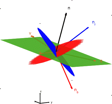
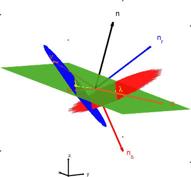
Figures 1-3 illustrate the process involved in the extended imaging condition and describe pictorially its physical meaning. Figure 1 shows the source and receiver planes, as well as the reflector plane together with their unit vector normals. Figure 2 shows the source and receiver planes displaced by the space lag vector ${\boldsymbol {\lambda }}$ contained in the reflector plane, as indicated by equation 18. The displaced planes do not intersect at the reflection plane, thus they do not contribute to the extended image at this point. However, with the application of time shifts with the quantity $\tau =\left ({\bf q}\cdot {\boldsymbol{\lambda}} \right)\sin\theta/v$ , i.e. a translation in the direction of plane normals, the source and receiver planes are restored to the image point, thus contributing to the extended image, Figure 3.

eicawfl
Figure 1. The reflector plane (of normal ${\bf n}$ ), together with the source and receiver planes (of normals ${\bf n}_s$ and ${\bf n}_r$ , respectively). The figure represents the source/receiver planes in their original position, i.e. as obtained by wavefield reconstruction.

eicxshift1
Figure 2. The reflector plane (of normal ${\bf n}$ ), together with the source and receiver planes (of normals ${\bf n}_s$ and ${\bf n}_r$ , respectively). The figure represents the source/receiver planes displaced with the space-lag ${\boldsymbol {\lambda }}$ constrained in the reflector plane.

eictshift1
Figure 3. The reflector plane (of normal ${\bf n}$ ), together with the source and receiver planes (of normals ${\bf n}_s$ and ${\bf n}_r$ , respectively). The figure represents the source/receiver planes displaced with space-lag ${\boldsymbol {\lambda }}$ and time-lag $\tau$ . The space and time-lags are related by equation 17.

Wide-azimuth angle gathers for wave-equation migration