New insights into one-norm solvers from the Pareto curve

Pareto curve

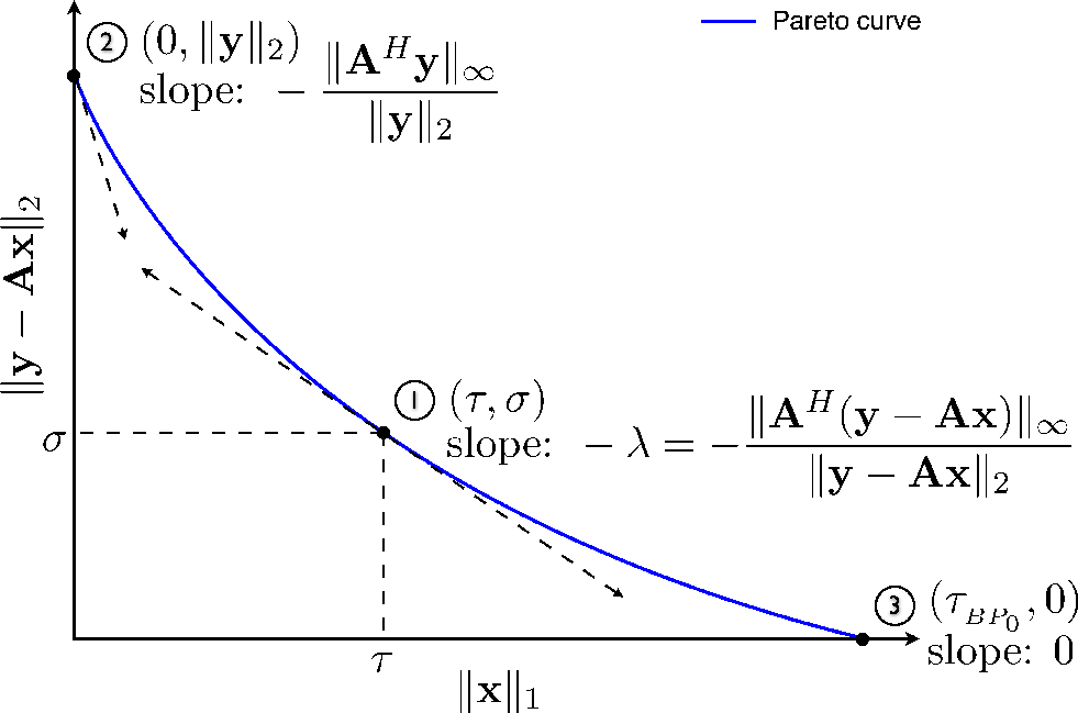
Figure 1 gives a schematic illustration of a Pareto curve. The curve traces the optimal tradeoff between $\Vert\ensuremath{\mathbf{y}}-\tensor{A}\ensuremath{\mathbf{x}}\Vert _2$ and $\Vert\ensuremath{\mathbf{x}}\Vert _1$ for a specific pair of $\tensor{A}$ and $\ensuremath{\mathbf{y}}$ in equation 1. Point clarifies the connection between the three parameters of QP$_\lambda$ , BP$_\sigma$ , and LS$_\tau$ . The coordinates of a point on the Pareto curve are $(\tau,\sigma)$ and the slope of the tangent at this point is $-\lambda$ . The end points of the curve--points and --are two special cases. When $\tau = 0$ , the solution of LS$_\tau$ is $\ensuremath{\mathbf{x}}=0$ (point ). It coincides with the solutions of BP$_\sigma$ with $\sigma=\Vert\ensuremath{\mathbf{y}}\Vert _2$ and QP$_\lambda$ with $\lambda=\Vert\tensor{A}^H\ensuremath{\mathbf{y}}\Vert _\infty/\Vert\ensuremath{\mathbf{y}}\Vert _2$ . (The infinity norm $\Vert\cdot\Vert _\infty$ is given by $\max\left(\vert\cdot\vert\right)$ .) When $\sigma =0$ , the solution of BP$_\sigma$ (point ) coincides with the solutions of LS$_\tau$ , where $\tau$ is the one norm of the solution, and QP$_\lambda$ , where $\lambda=0^+$ --i.e., $\lambda$ infinitely close to zero from above. These relations are formalized as follows in van den Berg and Friedlander (2008):

Result 1   The Pareto curve i) is convex and decreasing, ii) is continuously differentiable, and iii) has a negative slope $\lambda=\Vert\tensor{A}^H\ensuremath{\mathbf{r}}\Vert _\infty/\Vert\ensuremath{\mathbf{r}}\Vert _2$ with the residual $\ensuremath{\mathbf{r}}$ given by $\ensuremath{\mathbf{y}}-\tensor{A}\ensuremath{\mathbf{x}}$ .

For large-scale geophysical applications, it is not practical (or even feasible) to sample the entire Pareto curve. However, its regularity, as implied by this result, means that it is possible to obtain a good approximation to the curve with very few interpolating points, as illustrated later in this letter.

pcurve
Figure 1. Schematic illustration of a Pareto curve. Point exposes the connection between the three parameters of QP$_\lambda$ , BP$_\sigma$ , and LS$_\tau$ . Point corresponds to a solution of BP$_\sigma$ with $\sigma =0$ .

New insights into one-norm solvers from the Pareto curve