next up previous [pdf]

Next: Examples Up: Sripanich et al.: Wave-vector Previous: Locating singularities

Numerical algorithm

We can summarize the steps of the proposed elastic wave-vector decomposition as follows:
leftmargin=*
Considering the decomposition operator given in equation 14, we define each component of the decomposed wavefield corresponding to $ \alpha$ wave mode as
$\displaystyle \widetilde{U}^{\alpha}_x = A^{\alpha}_{xx} \widetilde{U}_x + A^{\alpha}_{xy}\widetilde{U}_y + A^{\alpha}_{xz} \widetilde{U}_z~,$     (26)
$\displaystyle \widetilde{U}^{\alpha}_y = A^{\alpha}_{yy} \widetilde{U}_y + A^{\alpha}_{xy} \widetilde{U}_x + A^{\alpha}_{yz} \widetilde{U}_z~,$      
$\displaystyle \widetilde{U}^{\alpha}_{z} = A^{\alpha}_{zz} \widetilde{U}_z + A^{\alpha}_{xz} \widetilde{U}_x + A^{\alpha}_{yz} \widetilde{U}_y~,$      

where each $ A^{\alpha}_{ij}$ with $ i$ and $ j$ denoting different components $ x,~y,$ and $ z$ is given in equation 16.
leftmargiin=*
To implement the proposed filtering of singularities, we multiply each component by a weighting factor defined as

$\displaystyle \hat{A}^{\alpha}_{ij} = A^{\alpha}_{ij}~w(\nu,\tau)~,$ (27)

where $ w(\nu,\tau) =$   min$ \left(\frac{\sin(\frac{\nu}{3})}{\tau},1 \right)$ , $ \hat{A}^{\alpha}_{ij}$ denotes the modified version of $ A^{\alpha}_{ij}$ , which is used in equation 26, and $ \tau $ is a thresholding parameter. This filtering process results in small $ \hat{A}^{\alpha}_{ij}$ in places where the given phase direction $ \mathbf {n}$ is close to the direction of a singularity. Figure 6 shows how the weight $ w(\nu ,\tau )$ changes with respect to different values of $ \tau $ in the case of the example orthorhombic model.

orthos02 orthos01 orthos005
orthos02,orthos01,orthos005
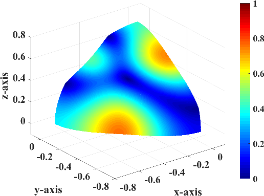
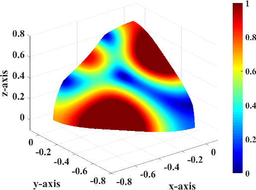
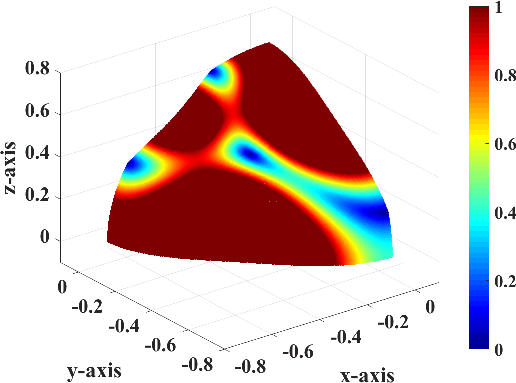
Figure 6.
Weight $ w(\nu ,\tau )$ in equation 27 with a) $ \tau =0.2$ , b) $ \tau =0.1$ , and c) $ \tau =0.05$ for the case of the example orthorhombic model.
[pdf] [pdf] [pdf] [png] [png] [png]

leftmargiiin=*
We then implement equation 26 with modified coefficients according to equation 27 applying the low-rank approximation as formulated in equation 18.
leftmargivn=*
As the last step, we compensate for the lost in amplitude information from the previous smoothing step using local signal-noise orthogonalization (Chen and Fomel, 2015) as described by

$\displaystyle \mathbf{U}^{\alpha}\mathbf{(x)} = \bigg(1+\Big\langle\frac{\mathb...
...^{\alpha}\mathbf{(x)}}\Big\rangle\bigg)\mathbf{U}^{\alpha}_{\tau}\mathbf{(x)}~,$ (28)

where $ \mathbf{U}^{\alpha}_{0}\mathbf{(x)}$ and $ \mathbf{U}^{\alpha}_{\tau}\mathbf{(x)}$ denote the separated wavefield without smoothing ($ \tau=0$ ) and with the specified smoothing respectively. $ \mathbf{U}^{\alpha}\mathbf{(x)}$ denotes the final separated wavefield after amplitude compensation and $ \langle\cdot\rangle$ represents a smooth division operator. The notion behind equation 28 is that the desired signal ( $ \mathbf{U}^{\alpha}_{\tau}\mathbf{(x)}$ ) is assumed to be locally orthogonal to the noise ( $ \mathbf{U}_{0}^{\alpha}\mathbf{(x)}-\mathbf{U}_{\tau}^{\alpha}\mathbf{(x)}$ ). Therefore, we can extract the remaining part of the signal in the noise--the missing amplitudes from the smoothing process--and simply add it back for the signal reconstruction.


next up previous [pdf]

Next: Examples Up: Sripanich et al.: Wave-vector Previous: Locating singularities

2017-04-18