 |
 |
 |
 | A reversible transform for seismic data processing |  |
![[pdf]](icons/pdf.png) |
Next: Conclusions
Up: Burnett & Ferguson: Reversible
Previous: NMO by Transform
Casting a theoretically continuous input signal as a vector is a natural way to view recorded seismic data.
The time-sampling interval of the recorded data determines the Nyquist frequency of the recorded signal (Gubbins, 2004), and it can be assumed that the data is frequency band-limited between zero and the Nyquist frequency (Gubbins, 2004).
This means that the recorded signal is exactly determined by this small and discrete range of frequencies.
No information is gained by using filters that operate on frequencies higher than the Nyquist frequency.
This observation, combined with the Fourier sampling theorem, suggests that a continuous, but band-limited form of the recorded signal exists, and it is exactly described by the Fourier basis.
This continuous form is not necessarily the same as the true continuous function that a seismometer attempts to record.
Conventional processing algorithms estimate the values of this continuous function by assuming that the function behaves like some interpolant between samples.
A repeatable and accurate approach to discrete data processing is to return the exact value of the band-limited continuous equivalent of the recorded signal at any desired input coordinate.
The data processing transform does exactly this.
The data processing transform is a special case of the nonstationary Fourier shift theorem.
It follows then, for the continuous case, that data processing steps implemented by transform are effectively performing convolution with a shifting scaled Dirac delta function.
The sifting property of the delta function justifies using convolution with a delta function to extract the exact values of a continuous input function at exact target times.
This is the ideal way to apply data processing corrections in either transform or mapping approaches, but the discrete nature of seismic data prevents this.
By showing that interpolation operators are approximations to the Dirac delta function, we suggest that any interpolation scheme can be viewed as an approximation to a continuous and exact nonstationary shift.
The Dirac delta function can be formulated as the generalized limit of other more common functions (Papoulis, 1962).
Two clear examples of this are boxcar (rectangle) and Gaussian functions, which both approach an impulse as their widths go to zero and their heights go to infinity (Papoulis, 1962).
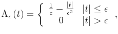
Take for example the boxcar function:
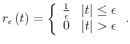 |
(28) |
As  approaches zero, the width of the boxcar goes to zero, and the height goes to infinity (see Figure 7).
As this occurs, the boxcar function approaches the Dirac delta function:
approaches zero, the width of the boxcar goes to zero, and the height goes to infinity (see Figure 7).
As this occurs, the boxcar function approaches the Dirac delta function:
 |
(29) |
The scaled boxcar function is used as an interpolant for nearest-neighbour interpolation, where the width of the boxcar is equal to the sampling interval.
This is a poor choice in most cases, as nearest-neighbour interpolation in the time domain, for example, has the unwanted effect of multiplying the frequency spectrum by a sinc function.
Conversely, nearest neighbour interpolation in the frequency domain introduces ringing into the time series.
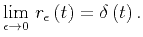
Linear interpolation is equivalent to convolution with a scaled triangle function with a width equal to twice the sampling interval (Harlan, 1982).
The triangle function also approaches the delta function as its width goes to zero and height goes to infinity:
 |
(30) |
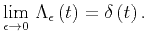 |
(31) |
This behaviour can be seen in Figure 8.
A more common interpolant used in seismic data processing is the sinc function.
Data processing corrections implemented by sinc-interpolation algorithms effectively perform convolution of the input signal with a shifting scaled sinc-function.
In the general continuous case, this has no clear justification, but for band-limited or discrete data, the purpose of the sinc-function becomes apparent.
The Fourier transform of the sinc-function is a boxcar function over its own frequency content (Harlan, 1982).
Since the ideal interpolant should not affect the frequency content of the data while it estimates an intermediate value, a sinc function with frequency content at least up to the Nyquist frequency of the input signal will be the ideal interpolant (Harlan, 1982).
Computational efficiency is often increased by truncating the length of the sinc operator (Harlan, 1982), and tapering of the truncated sinc function is often performed (Rosenbaum and Boudeaux, 1981) to reduce the Gibbs phenomena ringing.
The sinc function is a very good choice for an interpolant as it attempts to respect the finite bandwidth of the recorded data.
However, convolution with a sinc function is still an approximation to ideal continuous convolution with the delta function.
For the following expression (Elliot and Rao, 1982), as
approaches infinity, the normalized sinc function approaches an impulse (See Figure 9):
sinc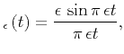 |
(32) |
 sinc sinc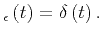 |
(33) |
There are more similarities between the narrowing sinc function and the Dirac delta function than just the shape of the pulse.
When
is less than infinity in 32, the side lobes of the sinc function mimic Gibbs phenomenon in Fourier transform theory (Papoulis, 1962).
Since the Fourier transform of a sinc function is a boxcar function, one can also visualize how it approaches the delta function in the Fourier domain.
As the sinc function narrows, its frequency content increases, and its boxcar Fourier transform broadens.
When the sinc function finally becomes an impulse, its Fourier spectrum is an infinitely wide boxcar, which is simply a constant, just as the Fourier transform of the delta function.
Applying a band-pass filter to a delta function yields a sinc function, and conversely, the sinc-function is a band-limited estimation of the Dirac delta function.
Therefore, the sinc-function interpolant, before truncation or tapering, respects the Fourier basis assumed by the Fourier transform, and is equivalent to processing by discrete nonstationary filtering.
The inverse to any processing step is exactly formulated here for the continuous case using the nonstationary version of the Fourier shift theorem.
This is not surprising, as even the conventional procedure of mapping data directly between input and output times is exactly reversible assuming continuous data.
Casting the integral kernel as a discrete matrix defined on the sampling intervals allows a precise method of approximating the exact continuous form assuming a Fourier basis.
|
|
|
|
| A reversible transform for seismic data processing | |
|
Next: Conclusions
Up: Burnett & Ferguson: Reversible
Previous: NMO by Transform
2013-07-26