Using IWAVE

Bibliography

Brown, D., 1984, A note on the numerical solution of the wave equation with piecewise smooth coefficients: Mathematics of Computation, 42, 369-391.

Cohen, G. C., 2002, Higher order numerical methods for transient wave equations: Springer.

Fehler, M., and P. J. Keliher, 2011, SEAM Phase I: Challenges of subsalt imaging in tertiary basins, with emphasis on deepwater gulf of mexico: Society of Exploration Geophysicists.

(eISBN=9781560802884, eBook catalog number 114E).

Fomel, S., 2009, Madagascar web portal: http://www.reproducibility.org, accessed 5 April 2009.

Levander, A., 1988, Fourth-order finite-difference P-SV seismograms: Geophysics, 53, 1425-1436.

Moczo, P., J. O. A. Robertsson, and L. Eisner, 2006, The finite-difference time-domain method for modeling of seismic wave propagation: Advances in Geophysics, 48, 421-516.

Muir, F., J. Dellinger, J. Etgen, and D. Nichols, 1992, Modeling elastic fields across irregular boundaries: Geophysics, 57, 1189-1196.

Symes, W. W., D. Sun, and M. Enriquez, 2011, From modelling to inversion: designing a well-adapted simulator: Geophysical Prospecting, 59, 814-833.

(DOI:10.1111/j.1365-2478.2011.00977.x).

Symes, W. W., and T. Vdovina, 2009, Interface error analysis for numerical wave propagation: Computational Geosciences, 13, 363-370.

Terentyev, I., and W. W. Symes, 2009, Subgrid modeling via mass lumping in constant density acoustics: Technical Report 09-06, Department of Computational and Applied Mathematics, Rice University, Houston, Texas, USA.

Terentyev, I., T. Vdovina, X. Wang, and W. W. Symes, 2012, IWAVE: a framework for wave simulation: http://www.trip.caam.rice.edu/software/iwave/doc/html/index.html, accessed 21 Sept 2012.

Virieux, J., 1984, SH-wave propagation in heterogeneous media: Velocity stress finite-difference method: Geophysics, 49, 1933-1957.

----, 1986, P-SV wave propagation in heterogeneous media: Velocity stress finite-difference method: Geophysics, 51, 889-901.

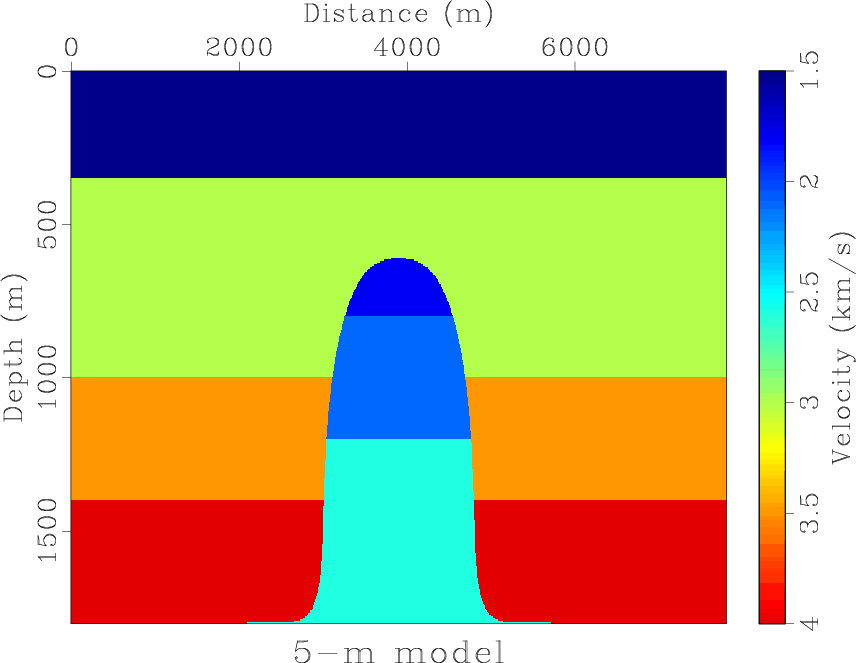
vp1
Figure 1. Dome velocity model

dn1
Figure 2. Dome density model

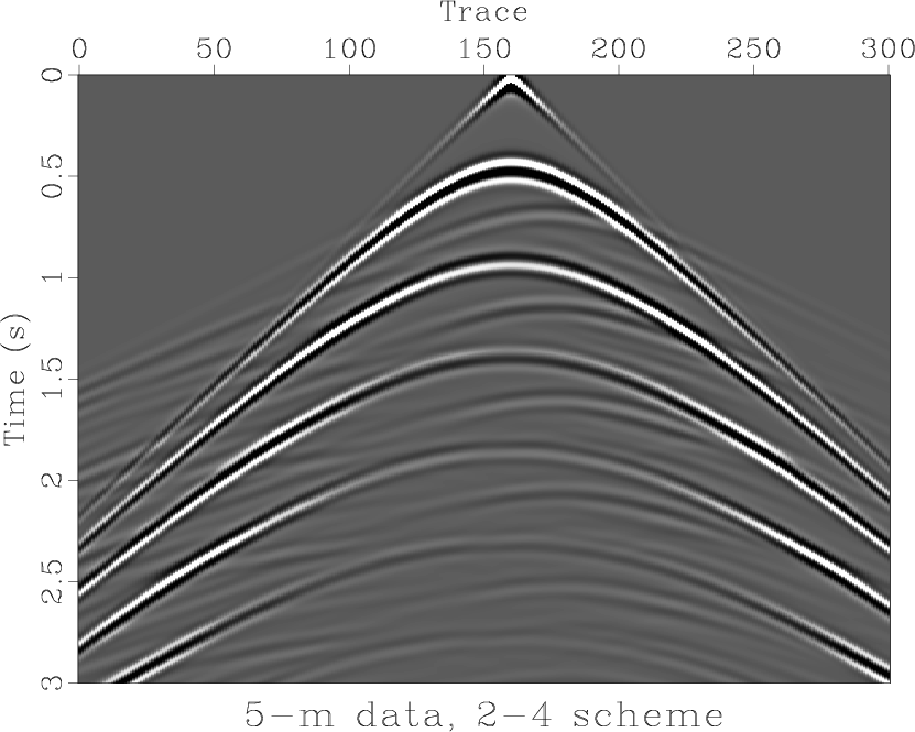
data1
Figure 3. 2D shot record, (2,4) staggered grid scheme, $\Delta x = \Delta z =$ 5 m, appropriate $\Delta t$, 301 traces: shot x = 3300 m, shot z = 40 m, receiver x = 100 - 6100 m, receiver z = 20 m, number of time samples = 1501, time sample interval = 2 ms. Source pulse = zero phase trapezoidal [0.0, 2.4, 15.0, 20.0] Hz bandpass filter.

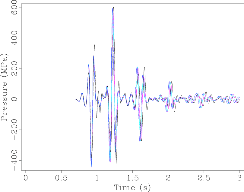
trace
Figure 4. Trace 100 (receiver x = 2100 m) for $\Delta x = \Delta z =$ 20 m (black), 10 m (blue), 5 m (green), and 2.5 m (red). Note arrival time discrepancy after 1 s: this is the interface error discussed in (Symes and Vdovina, 2009). Except for the 20 m result, grid dispersion error is minimal.

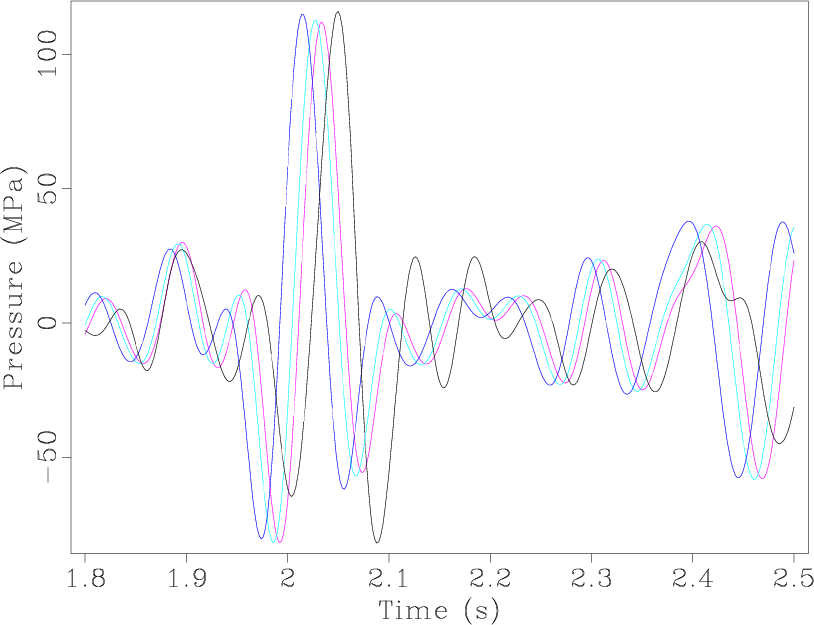
wtrace
Figure 5. Trace 100 detail, 1.8-2.5 s, showing more clearly the first-order interface error: the time shift between computed events and the truth (the 2.5 m result, more or less) is proportional to $\Delta t$, or equivalently to $\Delta z$.

data8k1
Figure 6. 2D shot record, (2,8) scheme, other parameters as in Figure 3.

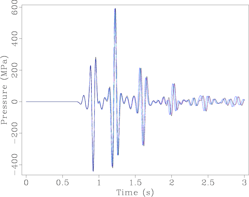
trace8k
Figure 7. Trace 100 computed with the (2,8) scheme, other parameters as described in the captions of Figures 3 and 4.

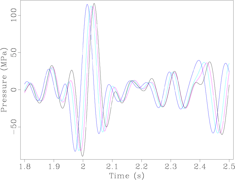
wtrace8k
Figure 8. Trace 100 detail, 1.8-2.5 s, (2,8) scheme.. Comparing to Figure 5, notice that the dispersion error for the 20 m grid is considerably smaller, but the results for finer grids are nearly identical to those produced by the (2,4) grids - almost all of the remaining error is due to the presence of discontinuities in the model.

Using IWAVE